SparklingTree: 30-40% faster speculative decoding over DSpark
TLDR: By combining first-order markov correction (DSpark), DDTree (tree based block diffusion draft speculative decoding), and a best-first search approximation, we create a speculator called SparklingTree. SparklingTree has a +32.7% increase in acceptance at budget 64 (+31.2% wall clock speedup), and +47.4% acceptance at budget 256 (+43.9% wall clock) over DSpark.
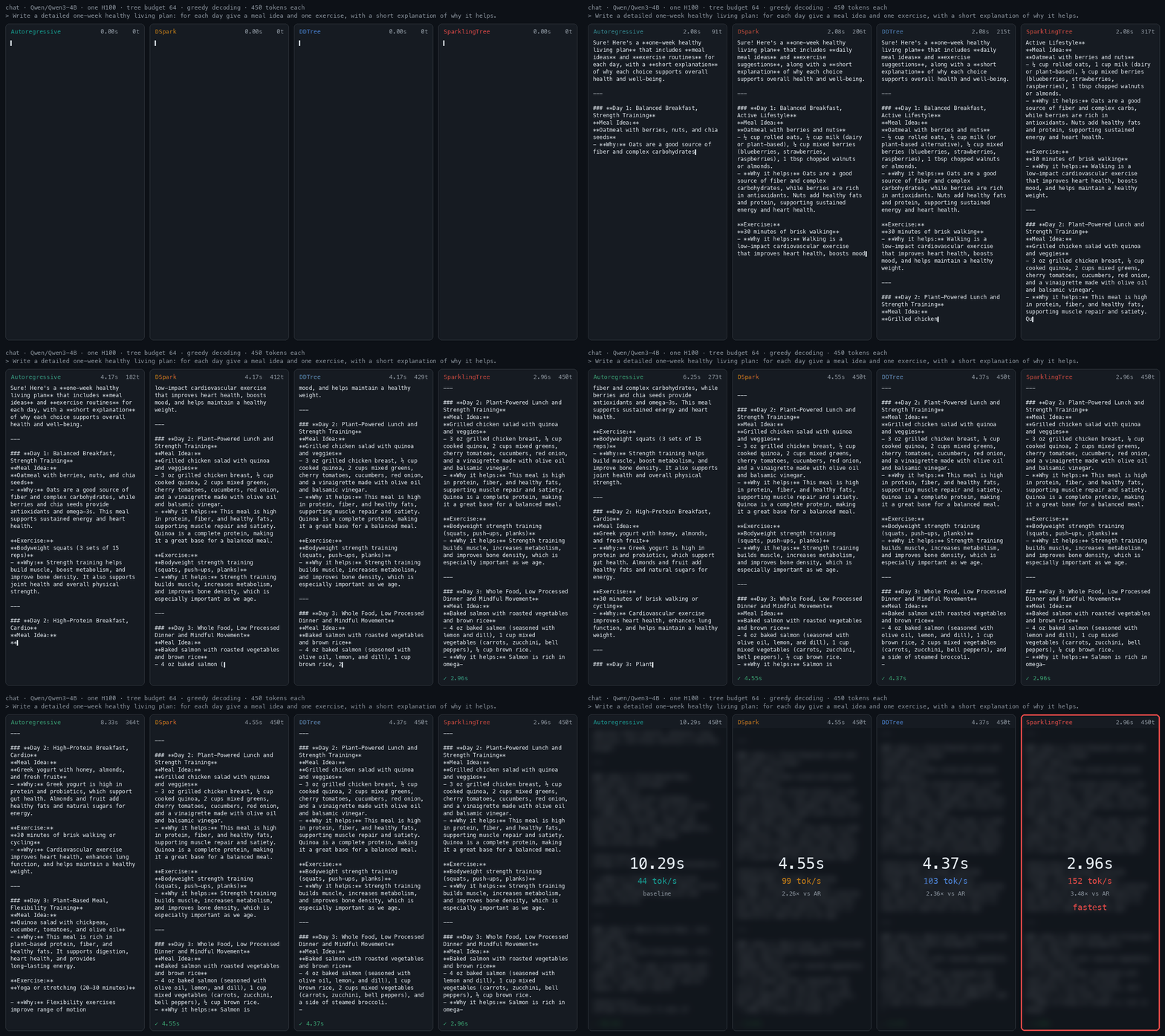
GitHub: jwlaboratory/sparkling-tree
Understanding DFlash
Speculative decoding is a method in which a draft (tiny) language model drafts multiple tokens at once, so that a target (large) model can verify multiple tokens at once (parallel) instead of one at a time. For more information, you should read this article: Speculative decoding from first principles.
Traditionally, speculative decoding has been done using autoregressive language models (step by step generation, like ChatGPT or Claude). Over time, advancements from MTP to Medusa to Eagle led to higher and higher acceptance lengths. To increase the max amount of drafted tokens, we would increase the amount of work by a linear factor, since the model is autoregressive. Actually, it'd be even more than linear, since attention is an $O(n^2)$ operation that grows as the number of tokens increases.
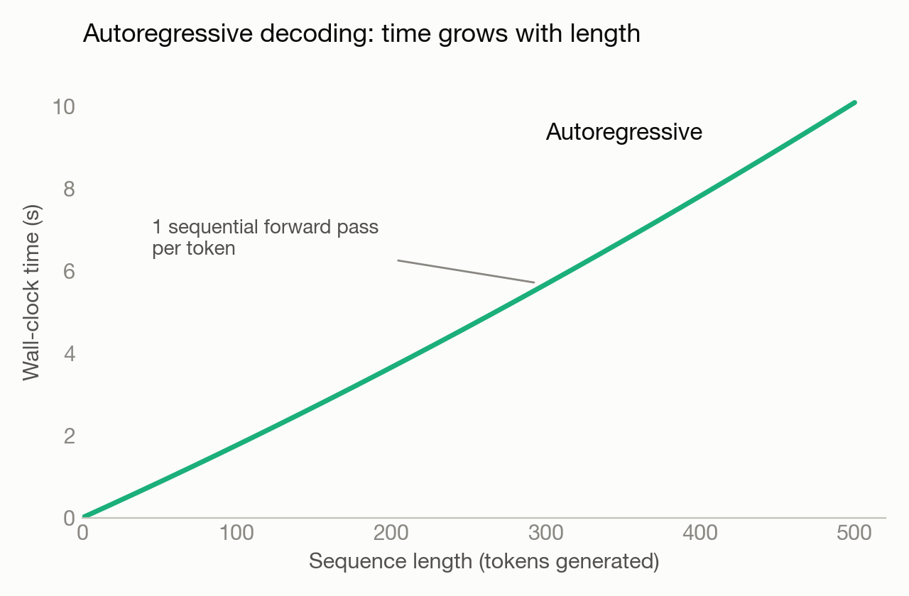
Suddenly, the "free drafter" does not look like a free drafter, even though acceptance lengths are high. This motivates DFlash.
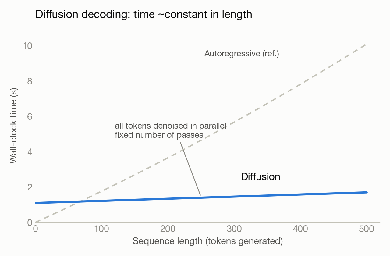
DFlash uses a block level diffusion draft model, instead of an autoregressive language model. This means that instead of creating one token at a time, DFlash "denoises" an entire block in parallel. (For diffusion models, increasing the number of tokens generated does not increase the latency, while it may reduce quality of the drafter.)
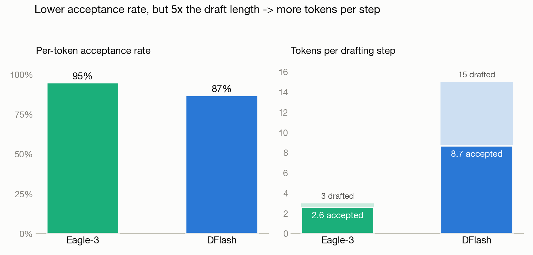
While the quality of the entire DFlash is lower (lower acceptance rate), it can draft 15 tokens instead of traditional drafters, i.e. Eagle3 (drafting just 3 at a time).
DFlash creates a matrix of marginal probabilities that is sampled from and used as the drafted token for the target. We'll see how this is important in the next section. You can visualize this as a table with Vocab columns and draft block size rows.
DFlash brings huge speedups, however we'll discuss more of the limitations of DFlash in the following 2 sections.
DFlash Paper: arxiv.org/pdf/2602.06036
Understanding DDTree
Earlier, I explained that DFlash outputs a table with Vocab columns and draft block size rows. Each row is completely independent of each other (this is called marginal in statistics).
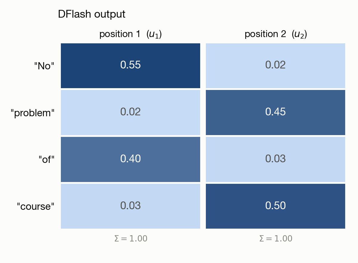
The key insight of the DDTree paper is that we can use these independent marginals to construct not just a single path or single solution, but a tree of solutions. Whenever the confidence of the drafter is low, we can branch into 2 paths and we will capture a higher success probability. While the paths are more shallow, it will have a higher overall acceptance rate.
For each node $u$ in the draft tree $T$, let $X_u \in \lbrace 0, 1 \rbrace$ indicate whether $u$ is accepted. A node is accepted only if every token on the chain from the root down to $u$ is accepted, so the number of accepted tokens is $\sum_{u \in T} X_u$. By linearity of expectation (which holds even when the $X_u$ are dependent):
where $\mathrm{path}(u)$ is the chain from the root to $u$ (inclusive), and $q(v)$ is the per-token acceptance probability, so the product is the prefix probability that the entire chain up to $u$ survives verification.
Let's compare two different ways of doing this: chain vs tree.
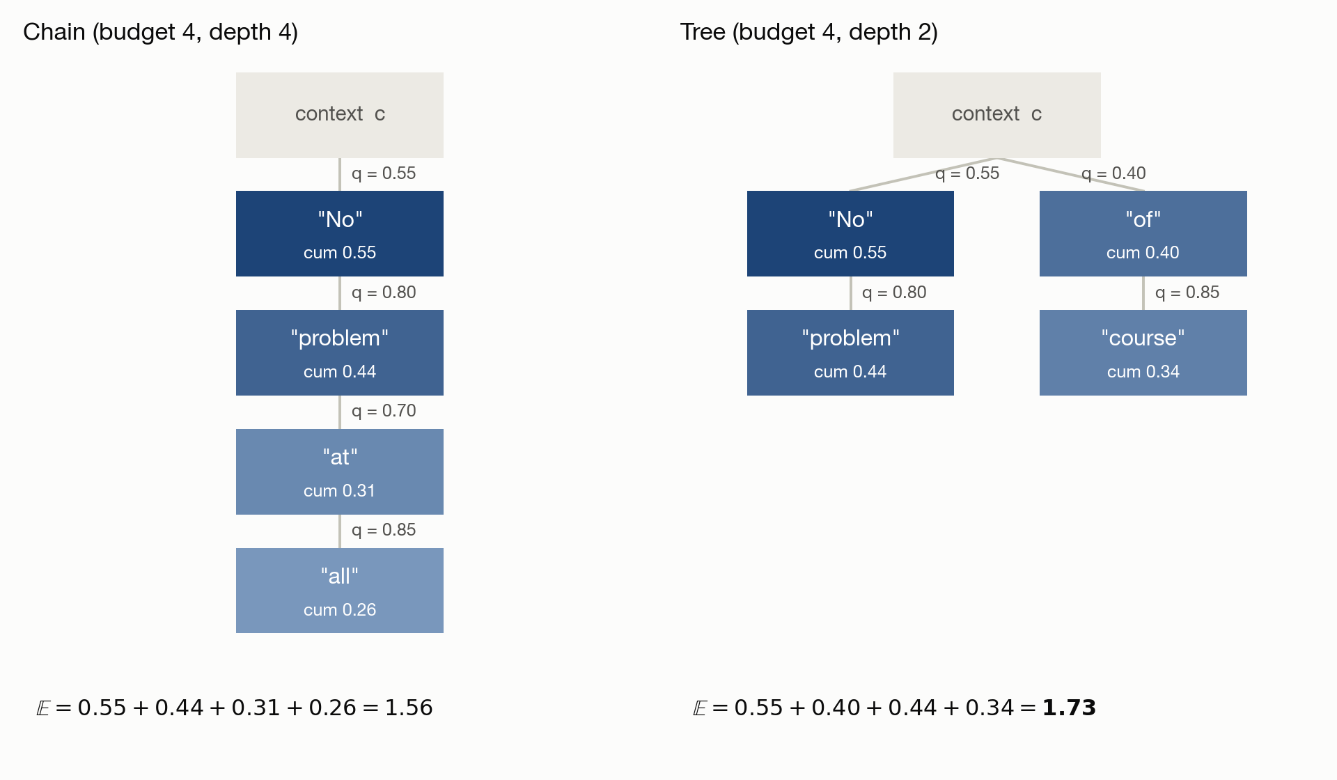
Here you can see the sum of the chain has an expected value of:
However the sum of the tree has an expected value of:
Clearly, the tree even though being much shallower has a higher expected value (even at the same total token budget). The cost of the tree is the cost of creating and verifying more tokens. DDTree mitigates much of this in the way it creates the tree and its tree attention mask, but at higher batch sizes the cost definitely weighs down on performance.
How is the tree actually created?
DDTree implements the tree creation and verification using a lazy best-first heap algorithm. It's important to understand how it works because in SparklingTree we have to modify this algorithm.
A max heap is a data structure that uses a tree. The heap keeps the max element at the top, and at each layer lower, strictly smaller items. You can push any element, and the heap will add it at $O(\log N)$ time. You can also take the top element out in $O(\log N)$ time as well because of the nature of tree operations. You can read about how max heaps work here: introduction to max heap.
Step 1: Sorting the DFlash marginals
The matrix shape is 15 rows (token guess at position 1, 2, … block size = 15) by vocab size (approx 152k columns). On GPU (torch.topk), it selects the top K logits of each row (K being the max token budget for the tree, because we can never take something outside the max token budget anyway), and then runs torch.logsumexp to make each logit comparable, then finally sorts each row.
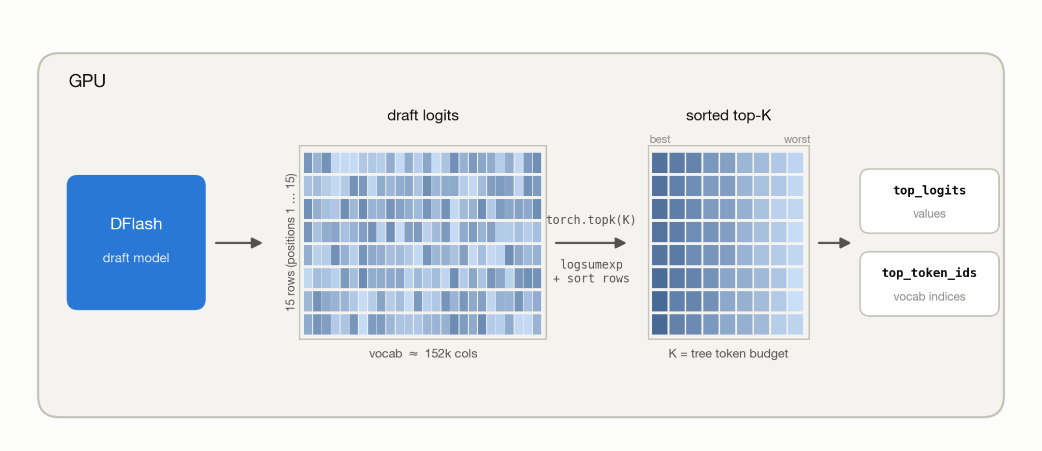
Since it's relatively small and on GPU, it doesn't take much time to do this compute. It creates 2 vectors: top_logits (the values), and top_token_ids (indices into vocab). We needed to sort so the following sequential steps are much faster.
The code from the official DDTree codebase (github.com/liranringel/ddtree) that does this sorting on GPU:
topk = min(budget, draft_logits.shape[-1])   # how many to sample (top-K) per row
depth_limit = int(draft_logits.shape[0])      # horizontal length; cannot go deeper than this
logits = draft_logits.float()
top_logits, top_token_ids = torch.topk(logits, k=topk, dim=-1)
log_z = torch.logsumexp(logits, dim=-1, keepdim=True)Step 2: Copy this over to the CPU
Next, the GPU sends these values to the CPU. Since the actual tree generation involves building a heap (sequential) and lookup tables, it's much better suited for the CPU rather than the device/GPU.
The cost of this is that we need to do a device to host synchronization, causing blockades and transfer costs between CPU and GPU. This is clearly bad, but the DDTree authors outweigh this synchronization with the benefits of the tree. To learn more about this, read this article by @charles_irl: host overhead and inference efficiency.
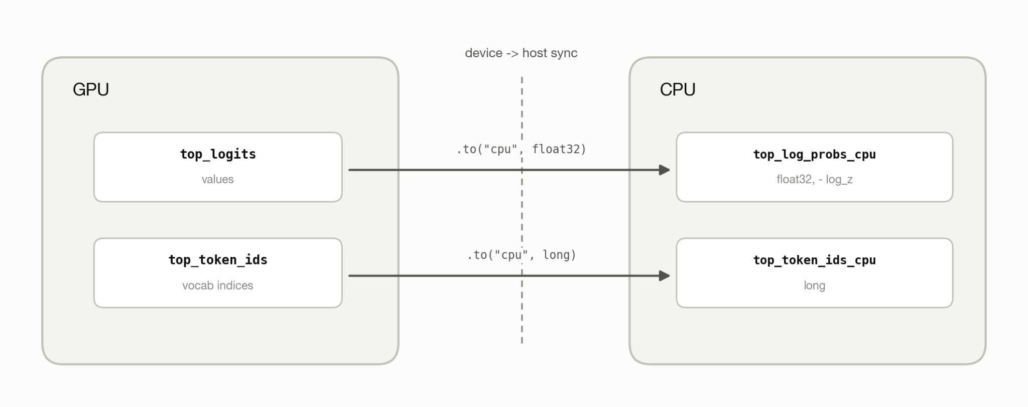
top_log_probs_cpu = (top_logits - log_z).to(device="cpu", dtype=torch.float32)
top_token_ids_cpu = top_token_ids.to(device="cpu", dtype=torch.long)
build_subtimes["tree_build_copy"] = cuda_time() - copy_startStep 3: The best-first heap algorithm
The algorithm will pop the top element in the heap (highest probability cumulative path) so far. Then, add the next highest probability sibling (explore horizontally), and the highest probability child (explore deeper), back into the heap.
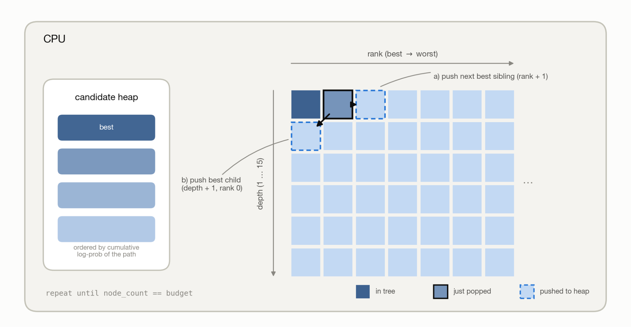
It does this sequentially until it has popped enough elements to reach the node budget. The algorithm guarantees you will capture the highest total expected value. You can read more about the algorithm here: best-first search.
while heap and node_count < budget:
    _, ranks, parent_index, depth, rank, logw = heapq.heappop(heap)

    token_id = int(top_token_ids_np[depth - 1, rank])
    current_index = node_count + 1
    node_token_ids_np[node_count] = token_id
    node_depths_np[node_count] = depth
    parents_np[current_index] = parent_index
    child_maps.append(dict())
    child_maps[parent_index][token_id] = current_index
    node_count += 1

    if rank + 1 < topk:
        sibling_ranks = ranks[:-1] + (rank + 1,)
        sibling_logw = logw - float(top_log_probs_np[depth - 1, rank]) + float(top_log_probs_np[depth - 1, rank + 1])
        heapq.heappush(heap, (-sibling_logw, sibling_ranks, parent_index, depth, rank + 1, sibling_logw))

    if depth < depth_limit:
        child_ranks = ranks + (0,)
        child_logw = logw + float(top_log_probs_np[depth, 0])
heapq.heappush(heap, (-child_logw, child_ranks, current_index, depth + 1, 0, child_logw))Step 4: Creating the tree mask
This part runs through the tree and creates a flattened indexed array that explains what the ancestor of each token is. This becomes useful during the speculative decoding verification step, because the GPU can do a single fat matrix multiplication instead of many small ones, because it knows exactly what tokens need to be computed relating to what other KV.
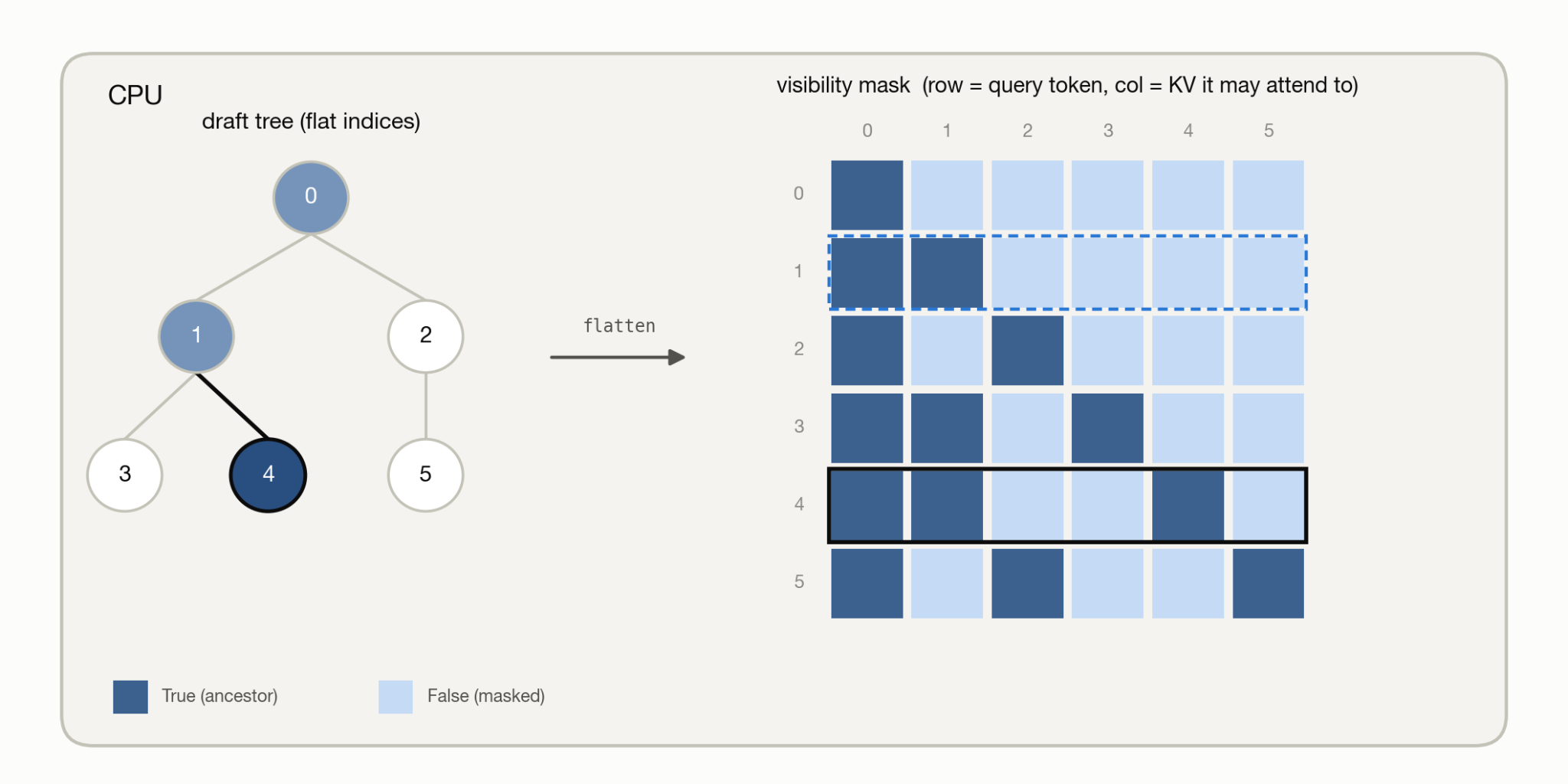
visibility_np = np.zeros((current_length, current_length), dtype=np.bool_)
visibility_np[0, 0] = True
for index in range(1, current_length):
    parent_index = int(parents_np[index])
    visibility_np[index, :index] = visibility_np[parent_index, :index]
    visibility_np[index, index] = True
build_subtimes["tree_build_visibility"] = time.perf_counter() - visibility_startOverall DDTree provably has a higher expected number of accepted tokens (assuming that the drafter's "confidence" per vocab is the expected probability of it being accepted), even at the same token budget. However, it comes at a cost: the creation of such a tree, the tree mask, CPU host sync overhead, and the weird matmul (jumping around a lot with the tree mask as opposed to a standard attention). DDTree generally is really good for extremely memory bound systems (low batch sizes), but starts to lose due to the overhead at higher batch sizes.
DDTree Paper: arxiv.org/pdf/2604.12989
Understanding DSpark
DSpark brings 2 new contributions to DFlash: first a confidence aware, hardware aware dynamic verification length, and second an autoregressive markov model head to align the marginals of DFlash. I'll quickly explain the former and focus on the latter because it is what we use in SparklingTree.
Confidence aware, hardware aware dynamic verification
DFlash always drafts the same amount of tokens but also verifies all of the tokens. This assumes that verification is parallel and free (which it somewhat is). However, at large batch sizes, when balancing compute bound and memory bound, having an infinite amount of tokens to verify eventually comes at compute costs and is no longer free.
To ride the compute bound / memory bound line even closer, DSpark adds 2 components to make the verification dynamic. First, a confidence head that uses the hidden state and previous token embedding and squashes it to a probability. They also add a calibration step to normalize against overconfident neural scores. Second, it profiles the hardware ahead of time into a throughput curve to figure out what the optimal amount of verification tokens is.
I didn't dig deep into this contribution from DSpark, so please correct me if I am wrong. SparklingTree doesn't build on this part of DSpark, but I think future work could definitely exploit the confidence or dynamic verification contribution.
First order markov model conditioning
The second contribution of DSpark is a small autoregressive head that helps align the diffusion drafter.
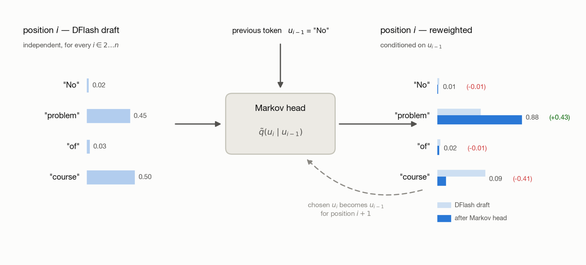
Let's see why this is useful, with a concrete (famous) example. Recall the DFlash output table from earlier: the two valid completions are "Of course" and "No problem", and the marginals at each position split their probability between them. This means that the sampling will sample "Of problem" or "No course" often. Because the DFlash model is a parallel diffusion model, each token is generated in parallel (with no knowledge of the previous token). Recall:
The probability at token position $i$ depends on context and noise, but not the previous token.
Recall that we switched from an autoregressive model (Eagle3) to DFlash because DFlash was faster at larger context lengths, despite bringing such parallel issues. DSpark's contribution is an "in between ground," in which the drafter is a semi-autoregressive, semi-parallel drafter that is both fast at a large number of generated tokens, but also conditioned on previous tokens.
The solution is to first draft in parallel like DFlash. Then, run a lightweight first-order markov model autoregressively to push the token distributions to be dependent on each other.
A first-order markov model (like a bigram table) is represented as a $V \times V$ matrix, where $V$ is vocab size. It shows, given the first token in the vocabulary, what the probability is of the next token being vocab index $0 \ldots V$.
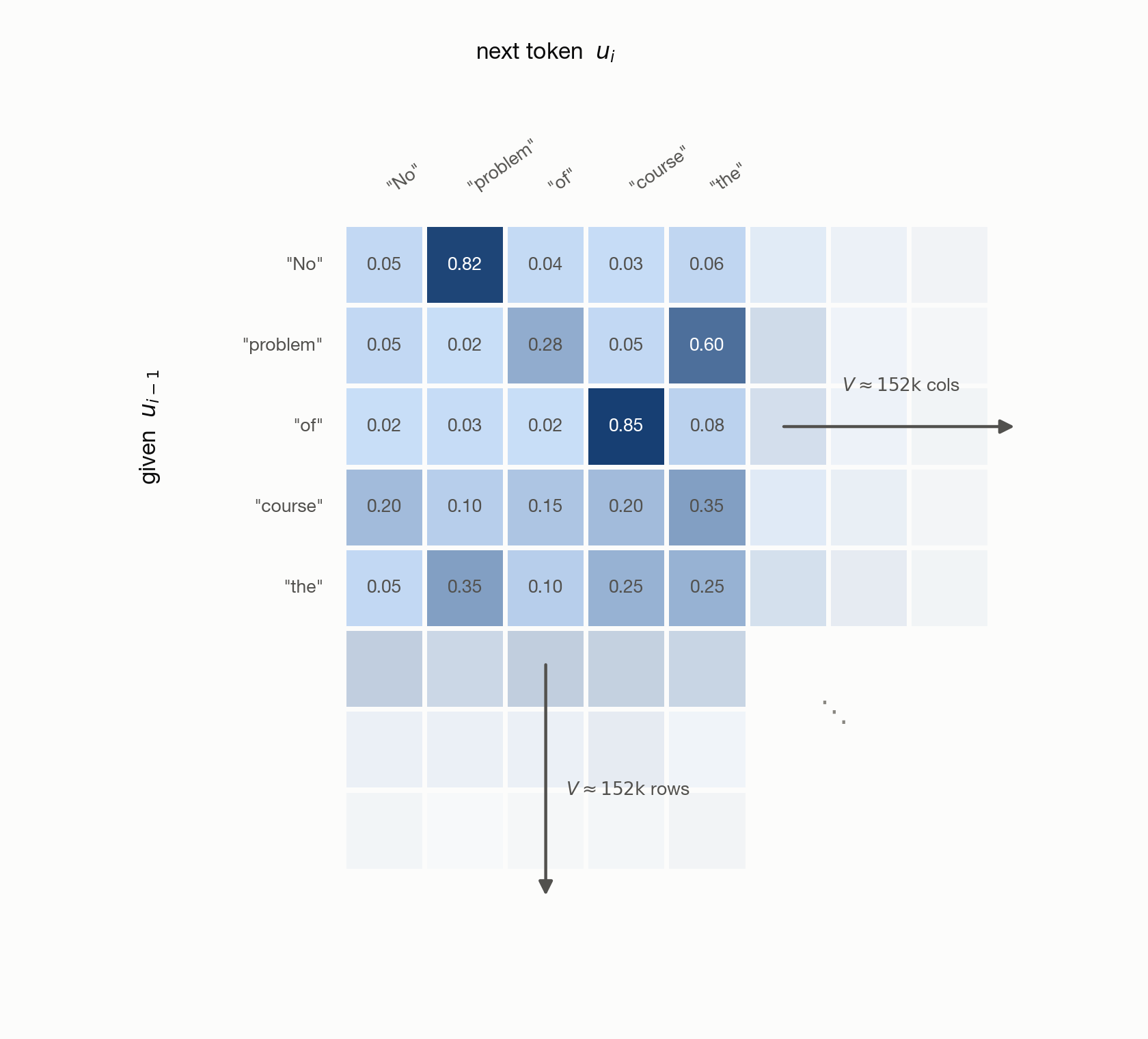
Given the vocab size for large models is in the hundreds of thousands, this makes it quite expensive to load into memory. If you increase the vocab size, you increase the parameters by a factor of $O(V^2)$.
Instead, DSpark uses a low rank factorization approximation. The intuition is that words come in groups. For example, following the word "the" or "a" is likely a noun. You don't need to know that individually "cat" follows "the", but rather that a group "noun" follows a group of words that look like "the" or "a". This is represented as two multiplications: first the "extraction", which squeezes the vocab into scores for $R$ groups, then the "projection", which projects each group into the words it connects to. $R$ is the rank, with a default of 256 unique groups.
You can see clearly: if $V$ is 100,000, then $100\text{k} \times 100\text{k}$ is much larger than the sum of $V \times 256 + 256 \times V$.
Now, DSpark uses the output of DFlash, selects the top token at index 0, runs the markov corrector, samples the top token at index 1, runs the markov corrector, and repeats in a loop. The markov corrector biases the sampling to make coherent sentences, and the fast parallel diffusion drafter makes high quality choices quickly.
Building SparklingTree
The DSpark paper shows an interesting insight. The chart below (taken from the DSpark paper) shows the per-position probability of acceptance. Note that this is not the cumulative probability, but the probability that position $i$ is accepted given that position $i-1$ was accepted.
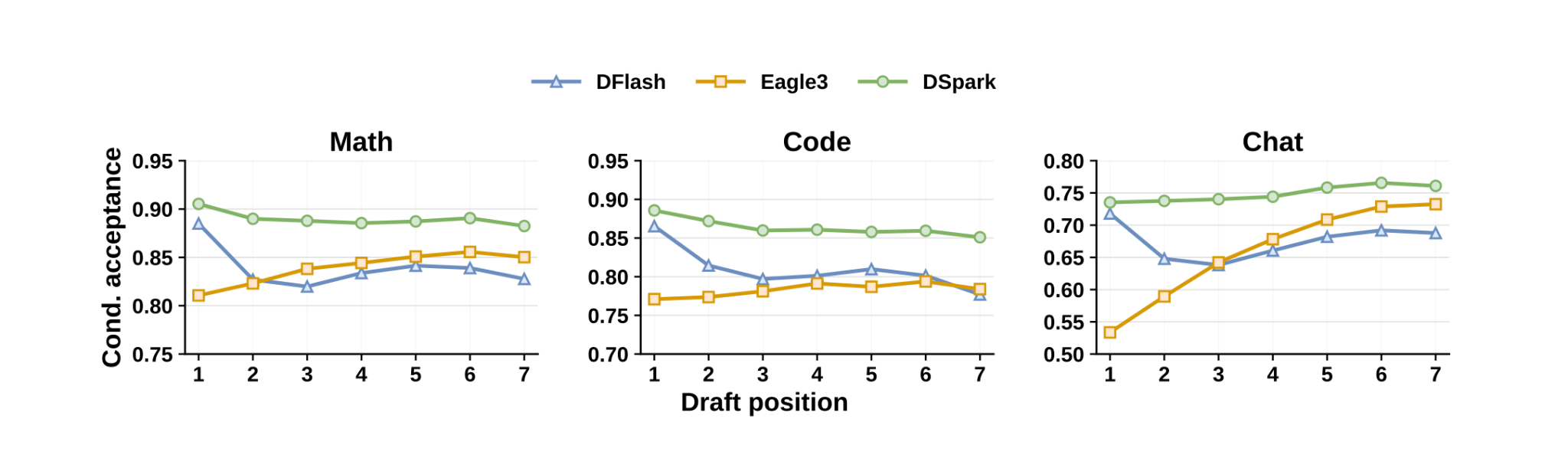
Here, especially in chat domains, we see that Eagle3 (autoregressive) is able to increase its acceptance probability over the positions. This is counterintuitive, but it's because if the autoregressive model finds its groove, it's likely to keep getting better over time. On the other hand, DFlash drops off a cliff over time, because the parallel diffusion model has the interference we discussed earlier. DSpark maintains a flat conditional acceptance by adding the lightweight autoregressive head.
At the same time, we saw that DDTree is able to bring much higher initial acceptance lengths to DFlash. This motivates us to try combining the parallel diffusion drafter to be fast (DFlash) + the autoregressive markov model to maintain acceptance at depth (DSpark) + trees to explore more branching nodes and get higher acceptance (DDTree). We call our idea "SparklingTree".
The rough outline for our initial naive SparklingTree is as follows:
- Draft using the diffusion drafter.
- Sort the first row (first index), push the top token onto the max heap.
- Pop the max token from the heap, put it on the tree.
- Run the autoregressive markov model on depth $i+1$ given depth $i$, sort the row, and push the top-probability child.
- Push the top-probability sibling (already sorted and conditioned).
- Repeat steps 3–5 until a full tree of max token budget is created.
We validated the idea by graphing the per-depth acceptance, now with SparklingTree included:
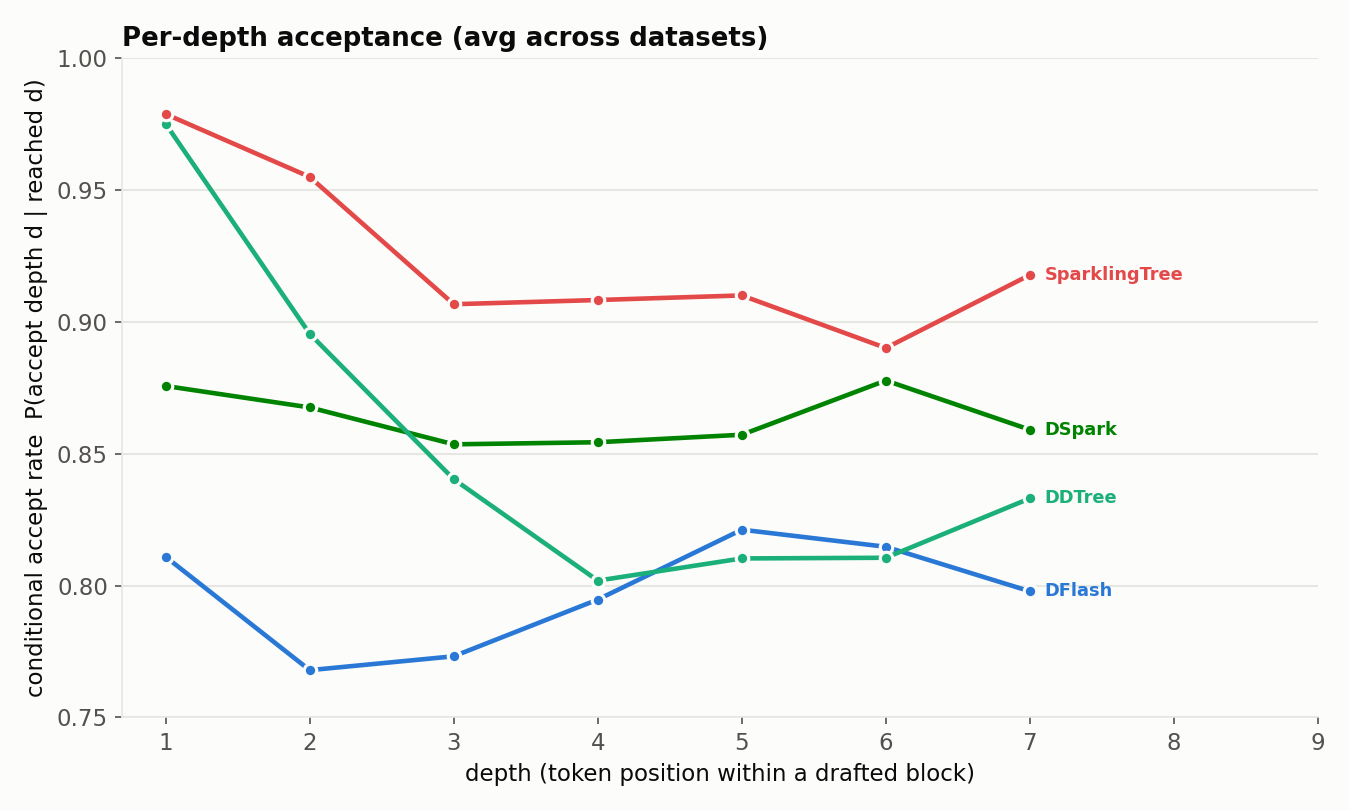
Note: we use the DDTree repository and the greedy decoding technique from its benchmarking scripts.
DDTree starts at an extremely high acceptance rate, because it can hedge with multiple shallow branches early, rather than go down one path that might be wrong entirely, as we predicted. On the other hand, DSpark starts lower, but because it has an autoregressive biaser, it stays steady (on sequences in which it starts correct, it is likely to continue being correct), while DDTree dips hard.
SparklingTree takes the best of both worlds. It starts high due to the hedging and branching, but also maintains relatively steady throughout depth because of the markov model conditioning.
Note: DDTree and DFlash are block size 16 drafters, so the graph continues for them, but not for this initial version of SparklingTree or DSpark.
We next compare the acceptance lengths of the different models:
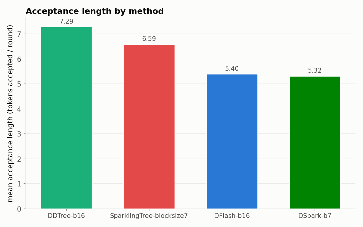
Here it seems that DDTree beats SparklingTree, but look closer: DSpark-b7 and SparklingTree-block7 are block size 7 models, compared to the block 16 models for DDTree and DFlash. This means DFlash is drafting 15 tokens at once, while DSpark is drafting only 7 (and SparklingTree is almost hitting the max ceiling at 6.59). You'll also see that the markov model + tree applied to DSpark leads to a +23.9% gain.
The harness must be trained jointly
You may wonder why we did not just use the DFlash model (since it is trained for block size 16) and drop it into the SparklingTree harness (DSpark markov model + tree). While the tree addition alone would work (DDTree works out of the box with DFlash, since it expects marginal probabilities), DSpark's markov model would not work.
The reason for this is that the markov model is trained jointly with the diffusion drafter. The objective of training DFlash is to make the top-probability tokens form a coherent sentence matching the target. The objective of training DFlash to work with the DSpark markov model is to train a model that generates probabilities that, after being corrected, create a coherent sentence.
To prove the point, we took the standard DFlash and added the markov model. We also took the DSpark model and took away the markov model. Clearly, the markov model only works when it was jointly trained.
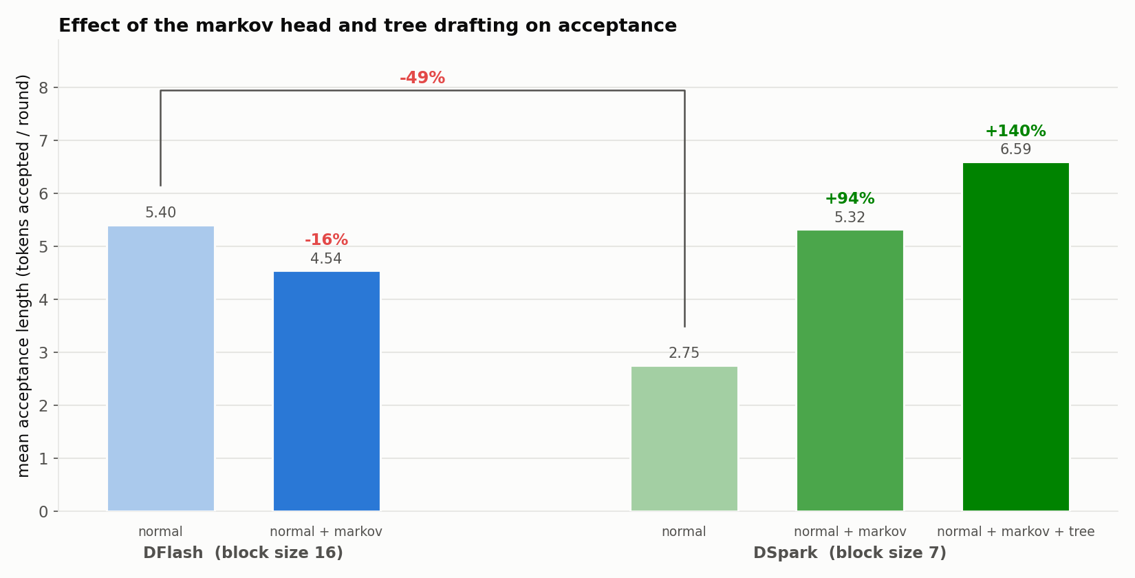
This gives us our first insight: the harness needs to be trained jointly with the model, or else it's not usable. This also means that for us to properly compare DFlash/DDTree (block size 16) against DSpark/SparklingTree (block size 7, nearly saturated), we'll need to train our own version of DSpark that is jointly trained for block size 16.
Extending the block size because SparklingTree saturated b=7
Like I explained earlier, the DSpark model + markov corrector + tree pushed DSpark to its max limit of 7 drafted tokens.
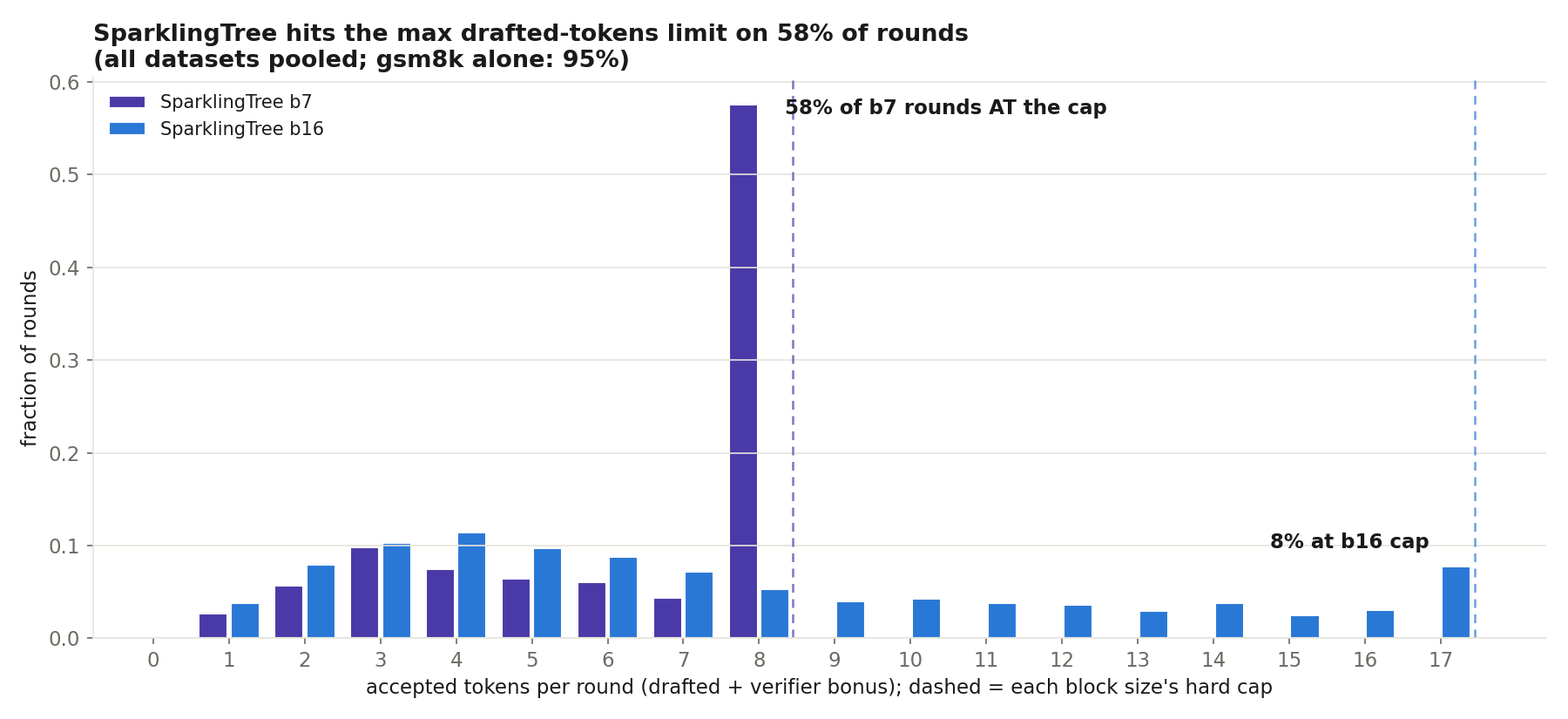
To break past this ceiling, we had to retrain DSpark to work with a block size of 15 (16 max tokens drafted and accepted). Since the starting model, DeepSeek's released dspark_qwen3_4b_block7 drafter, can be changed to draft 16 blocks with just a setting tweak (it does not change any parameter shapes), it can do block=16 out of the box, it just performs terribly because it has never seen training data above block=7.
We take the DeepSpec codebase, load in our starting point, then continue training with block size 16 on sequence size 768, 32 anchors per sequence, at 600 steps with 2,400 PerfectBlend chat conversations. We chose this dataset so as to not confound by training on the exact data we would test with. We also make sure to continue training the markov head (though it should not matter, since the markov model is position invariant) and the confidence head.
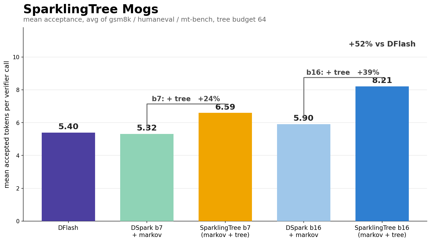
The results achieve our goal of smashing the 7 token max limit of DSpark. We also tested DSpark with our b16 but without the tree verification, to isolate that it wasn't just the extra training on PerfectBlend giving us the speedup, but rather the tree itself. The results show that at block size 16, the tree gives a 39% advantage, and at block size 7 a 24% advantage.
Our checkpoint: huggingface.co/shreybirmiwal/Qwen3-4B-DSpark-b16
The training recipe: experiment2-block16/training/ in the sparkling-tree repo
Measuring the wall clock speedup
We ran the algorithm using the DDTree benchmarking script and were surprised to see terrible speeds for the SparklingTree algorithm.
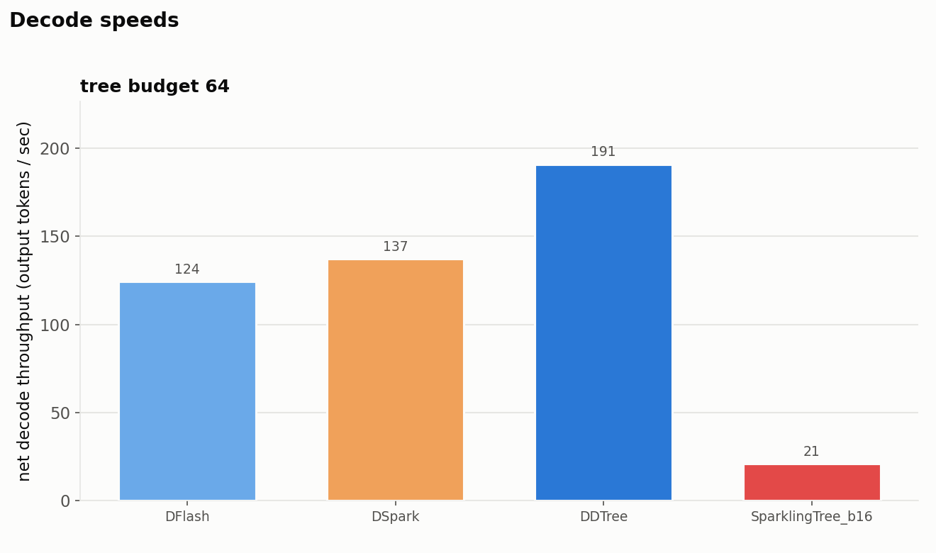
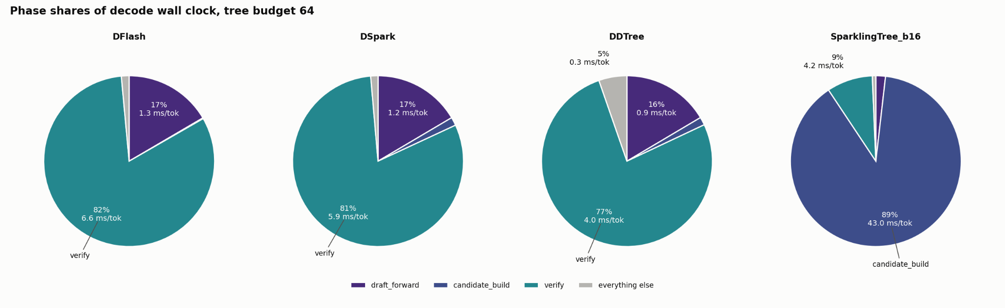
But why does it do so poorly? Clearly SparklingTree is accepting many more tokens. Investigating the time breakdown shows the story more completely:
| DFlash | DSpark | DDTree TB=64 | DDTree TB=256 | SparklingTree, B=16, Tree Budget = 64 | SparklingTree, B=16, Tree Budget = 256 | |
|---|---|---|---|---|---|---|
| Draft forward pass | 1.24 ms/committed-tok · 16.6% · 5.58 ms/round | 1.20 ms/committed-tok · 16.5% · 5.64 ms/round | 0.82 ms/committed-tok · 16.5% · 5.29 ms/round | 0.76 ms/committed-tok · 16.3% · 5.45 ms/round | 0.86 ms/committed-tok · 1.8% · 6.13 ms/round | 0.74 ms/committed-tok · 0.7% · 5.93 ms/round |
| Candidate tree construction | 0.01 ms/committed-tok · 0.1% · 0.05 ms/round | 0.11 ms/committed-tok · 1.6% · 0.54 ms/round | 0.08 ms/committed-tok · 1.5% · 0.49 ms/round | 0.12 ms/committed-tok · 2.7% · 0.89 ms/round | 41.93 ms/committed-tok · 88.8% · 299.34 ms/round | 107.75 ms/committed-tok · 96.0% · 860.21 ms/round |
| Verification by target model over candidates | 6.13 ms/committed-tok · 81.8% · 27.59 ms/round | 5.85 ms/committed-tok · 80.5% · 27.55 ms/round | 3.82 ms/committed-tok · 76.7% · 24.60 ms/round | 3.52 ms/committed-tok · 75.5% · 25.25 ms/round | 4.09 ms/committed-tok · 8.7% · 29.23 ms/round | 3.45 ms/committed-tok · 3.1% · 27.57 ms/round |
| Everything else | 0.11 ms/committed-tok · 1.5% · 0.49 ms/round | 0.10 ms/committed-tok · 1.4% · 0.47 ms/round | 0.26 ms/committed-tok · 5.3% · 1.71 ms/round | 0.25 ms/committed-tok · 5.5% · 1.83 ms/round | 0.31 ms/committed-tok · 0.7% · 2.23 ms/round | 0.29 ms/committed-tok · 0.3% · 2.31 ms/round |
| Total | 7.50 ms/committed-tok · 33.72 ms/round | 7.26 ms/committed-tok · 34.20 ms/round | 4.98 ms/committed-tok · 32.09 ms/round | 4.66 ms/committed-tok · 33.42 ms/round | 47.20 ms/committed-tok · 336.94 ms/round | 112.23 ms/committed-tok · 896.01 ms/round |
| accept/round (committed tokens per verify round) | 4.50 | 4.71 | 6.45 | 7.17 | 7.14 | 7.98 |
Observations
- Draft forward pass: The time per round is approximately the same. Draft forward is the time it takes for the diffusion draft model to do a forward pass, and it is approximately the same because they all share similar setups (4B-param diffusion drafters each doing one block forward per round). The time per committed token slightly varies (being fastest for SparklingTree) because it differs in accuracy (SparklingTree creates the most committed tokens).
- Candidate tree construction: The huge one. Let's get back to this one below.
- Verification by target model over candidates: Approximately the same. Of course the tree approaches have more nodes to verify, so it costs slightly more. Nuance 1: at larger batch sizes it is hard to say how this will change. I'm guessing it'll get worse once you pass the tip of the compute-bound ridge. At this point, being extremely memory bound (running batch size 1) under-shows the verification cost being the same (because all nodes are parallelized, and the bottleneck is the memory bandwidth loading in weights). Nuance 2: in MoE models it is hard to say how this will change as well. MoE models have to load in experts, so having more tree nodes to verify may trigger more experts to load in (which is bad, considering you are already memory bound).
What the heck is happening with the candidate tree construction?
Let's recall how the tree was constructed under DFlash, DDTree, DSpark, and now SparklingTree.
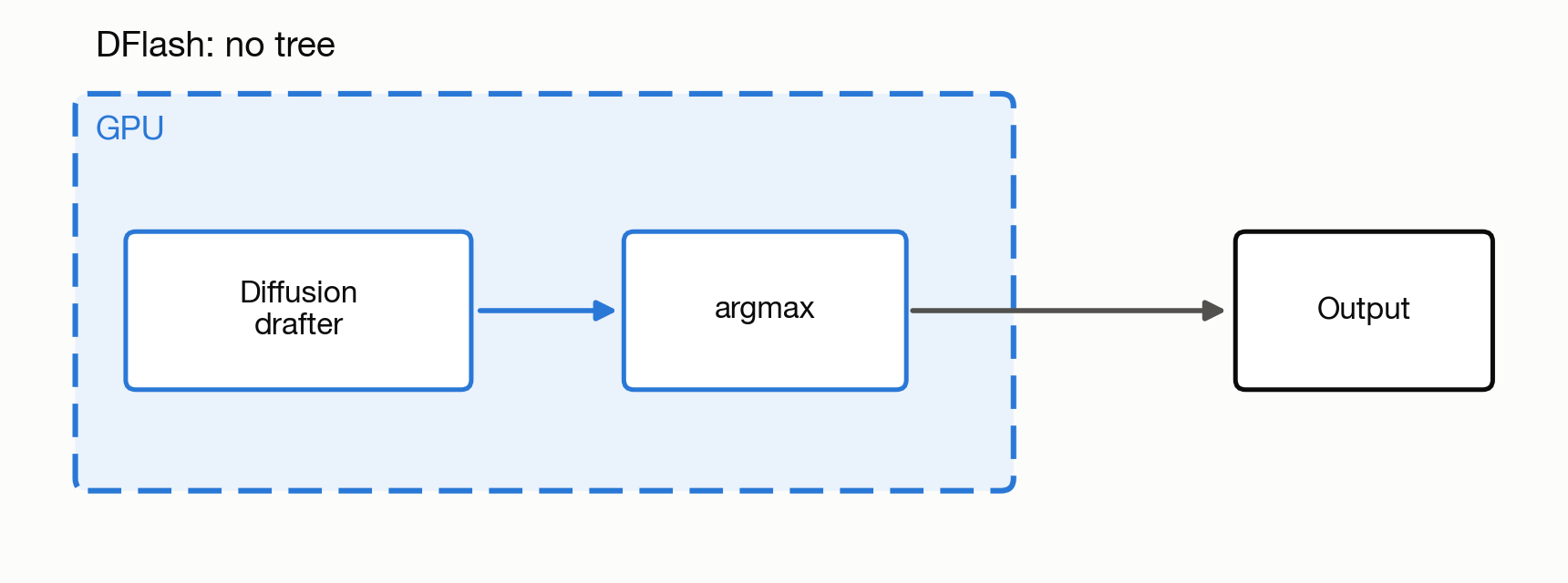
- DFlash: No tree at all. The diffusion drafter runs, then we take a singular GPU operation to get the top element at each index (argmax). The candidate construction is fastest (0.05 ms/round) because it is a singular GPU operation.
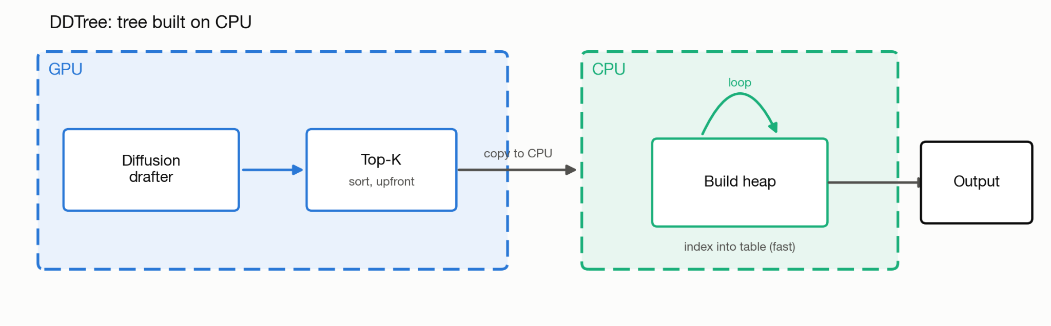
- DDTree: The diffusion drafter runs. We take a singular GPU operation to sort the top-k elements in each index (positions are independent, so this can be done upfront). One tiny table is copied over to the CPU, which iteratively builds a heap from this sorted table. The candidate construction is 0.49 ms/round, slower than DFlash due to the CPU working in a loop, but faster than the other speculators.
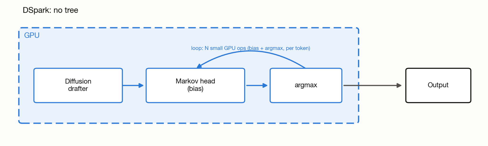
- DSpark: No tree at all. The diffusion drafter runs once. We then run the tiny autoregressive head on the GPU, bias the diffusion drafter, and sample the next token iteratively. DSpark is slightly slower (0.54 ms/round) than DDTree and DFlash because of the tiny autoregressive head: N small GPU operations have to occur rather than 1 big batched GPU operation.
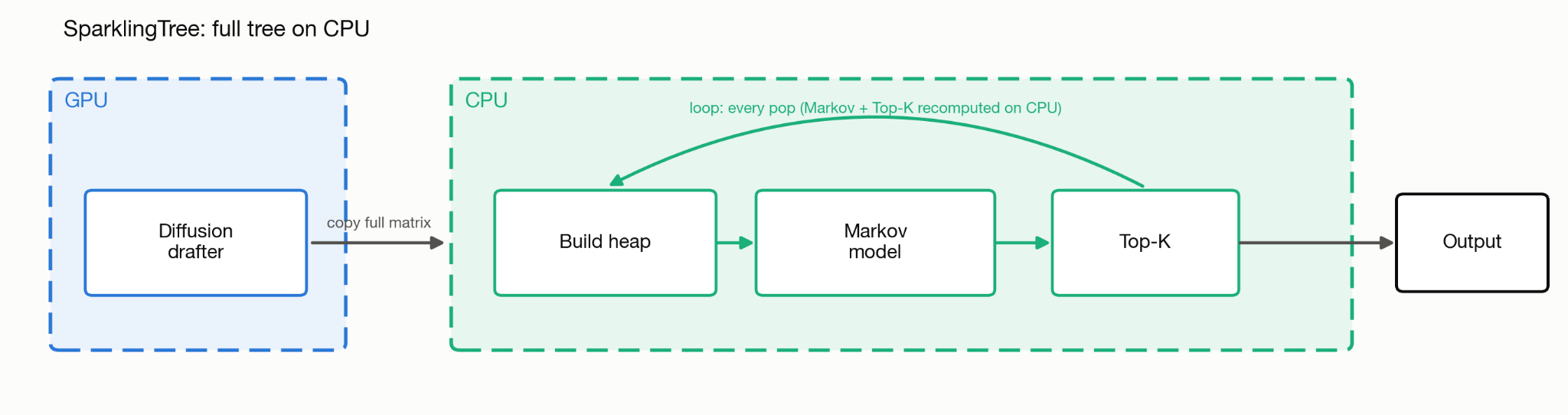
- SparklingTree: First, we create the diffusion draft matrix one time. Because the positions are no longer independent (markov model), top-k can no longer be precomputed upfront on the GPU. We have to first copy over the entire matrix to the CPU, which runs the heap algorithm from DDTree in a loop, but with the top-k computation + markov model running EVERY pop, and on CPU. It is by far the slowest at 299.34 ms/round.
Solving the candidate tree construction
Two key culprits are hitting us at the same time:
1. Transfer cost between CPU and GPU (the "prep" time)
We cannot go back and forth from CPU to GPU at each step. This means we can't just run the Markov model on the GPU and send results to the CPU to build the heap, because it'd take too much bandwidth (especially at batch sizes). So, we have to send all the compute to be done on the CPU. Additionally, we have to send the entire diffusion matrix (entire vocabulary size × block size) to the CPU.
The way we explore cutting this down is by running the top-k over all indexes immediately after the diffusion drafter is done (on GPU), before sending anything to the CPU. This could be lossy, because the markov bias is additive, so a token outside the base top-k could have been promoted into the true biased top-k that was excluded. It still captures ~99% because the bias is relatively small, so if we capture enough of a top-k (a few thousand instead of the 100k+ vocabulary size), we can practically cover it all.
We see a nearly 10× speedup by sending only the top-k of k=128 at node budget 64:
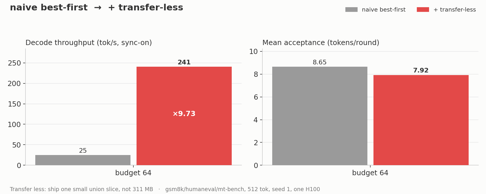
Surprisingly, BOTH the time to send the candidates to CPU (expected to decrease, because we send only a fraction of the full vocab size) AND the expansion time to create the heap (an unexpected side benefit) decreased significantly. The reason is that with a lower vocab size, the sorting and selecting task for the CPU becomes drastically faster as well.
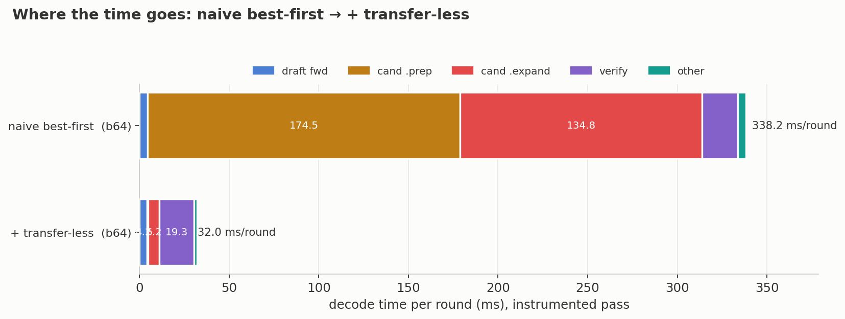
2. Doing repeated compute on CPU (particularly in the loop of expanding the tree)
When we were working with DDTree, we could do the computation of top-k all as one batched matmul on the GPU beforehand, because of the independence between indexes. Now, we have to do N small sorts all on CPU. (Multiple small serial operations, and on CPU, is not good.)
We need a way to be able to precompute as much of the iterative work in a single batch beforehand. Since it's only a first order markov model, it only needs to look back one token to determine the delta for the next token. Because of this, we can basically precompute into a table the entire (not low rank 2 multiplies) top-k markov model table upfront on the GPU and calculate the deltas at each depth upfront. Then, the CPU can simply do reads (no need to run the markov model each time or update the deltas and resort).
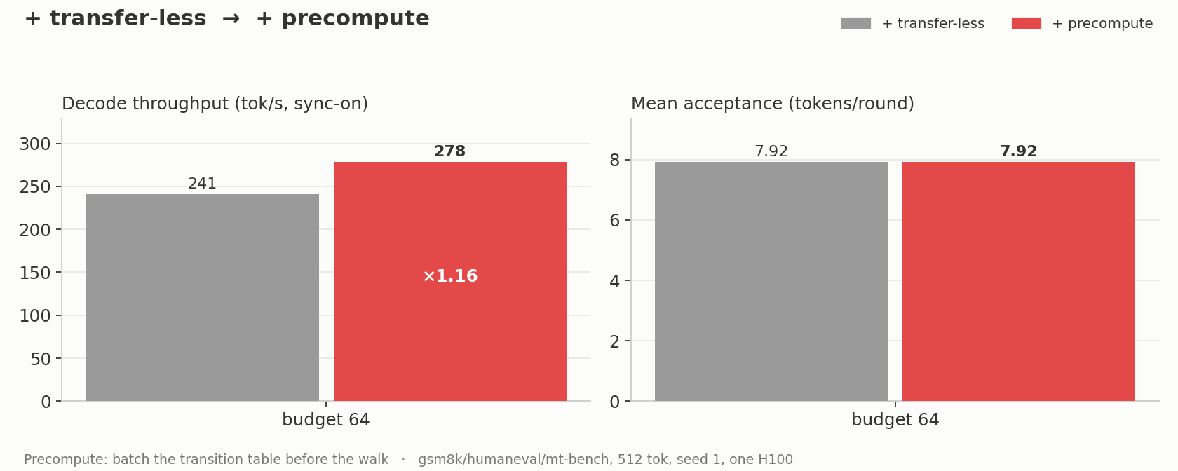
Even though we see a slight increase in the prep time (more compute upfront), the expansion (heap creation time) disappears almost entirely.
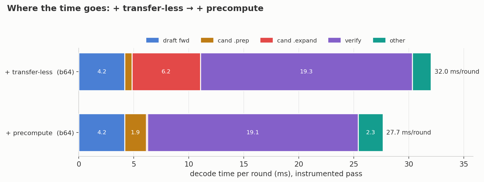
When comparing our final engineering results with DDTree, we see we are extremely competitive (and still leave room on the table for more work, i.e. fused kernels, beam search):
| Candidate construction (ms/round, budget 64, sync-on) | DDTree | SparklingTree |
|---|---|---|
| GPU table + one transfer (".prep") | 0.26 | 1.21 |
| CPU heap walk (".expand") | 0.12 | 0.15 |
| visibility mask | 0.04 | 0.04 |
| total candidate_build | ~0.5 | ~1.4 |
Conclusion and results
Using the DDTree paper benchmarking scripts (their setup of sync timing and their C++ KV compaction kernel enabled), we compare autoregressive, DFlash, DSpark, DDTree, and SparklingTree on six datasets spanning code (humaneval, mbpp), math (gsm8k, math500), and chat (mt-bench, alpaca), using a fresh random sample draw, 512-token generations, tree budgets {64, 128, 256}, greedy (temp 0) and sampling (temp 1.0), one H100, and all jobs on the same Modal GPU.
At node budget 64 and a top-k C=128, the results show SparklingTree at a 7.34 mean acceptance (+634% over autoregressive, +43.92% over DFlash, +32.73% over DSpark, +7.00% over DDTree), and a wall clock speedup of 4.29× (+329.62% over autoregressive, +36.31% over DFlash, +31.18% over DSpark, and +4.20% over DDTree).
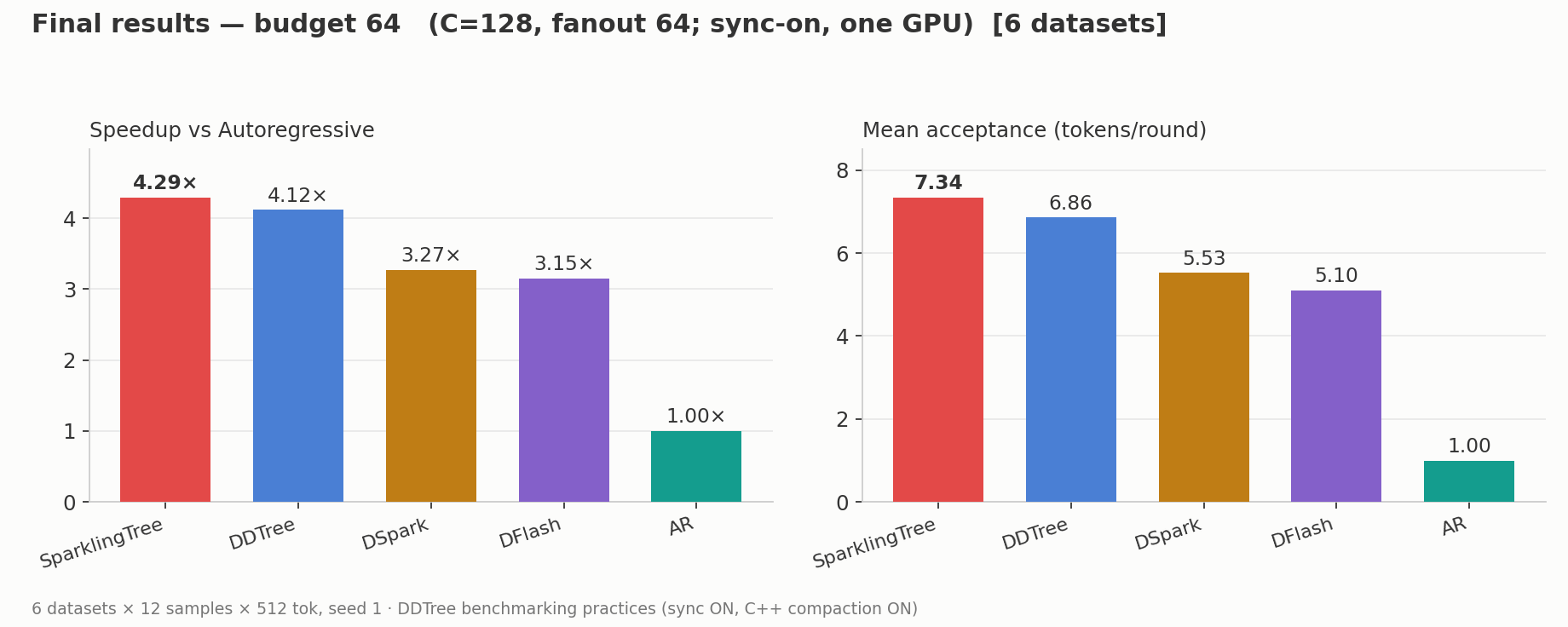
| budget 64 | mean acceptance | tok/s | speedup vs AR |
|---|---|---|---|
| Autoregressive | 1.00 | 52.0 | 1.00× |
| DFlash | 5.10 | 163.9 | 3.15× |
| DSpark | 5.53 | 170.3 | 3.27× |
| DDTree | 6.86 | 214.4 | 4.12× |
| SparklingTree | 7.34 | 223.4 | 4.29× |
At each domain, you can see SparklingTree generally edges out other methods, except for DDTree in hard domains such as math and coding:
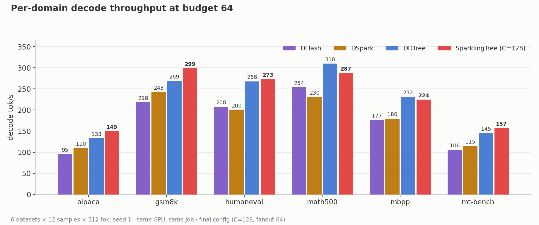
Perhaps this may be due to our training of the markov model at block size 16 on PerfectBlend. Definitely room to improve the markov model and the overall base DSpark model for block size 16.
Overall, over DSpark, we show huge gains in both speedups and acceptance:
| method | acceptance (tok/round) | decode tok/s | speedup vs AR |
|---|---|---|---|
| DSpark (chain, markov) | 5.53 | 170.3 | 3.27× |
| SparklingTree, budget 64 | 7.34 (+33%) | 223.4 (+31%) | 4.29× |
| SparklingTree, budget 128 | 7.73 (+40%) | 238.3 (+40%) | 4.58× |
| SparklingTree, budget 256 | 8.15 (+47%) | 245 (+44%) | 4.71× |
Future Ideas
- We saw that training the markov model jointly with the drafter is absolutely essential, otherwise accuracy collapses. Could it be that the tree should also be jointly baked into the training of the markov model + drafter?
- Similarly, DSpark has a confidence head. This was originally designed for a chain (NOT a tree), but can we still use it to help decide when to stop verification? This could make this project more viable at higher batch sizes. Additionally, how does it perform when it is jointly baked into the training as well? I did some cursory experiments in the archive-1 folder but didn't spend enough time to tell if this is an interesting direction.
- We run benchmarks at batch size 1 because the engineering lift to make this work on an engine like SGLang or vLLM would be too large. We should next try larger batch sizes. We guess that the gains likely diminish rapidly at larger batch sizes. Additionally: trying tensor-parallel GPUs, MoE models (more experts need to be loaded in, doing worse with the tree's extra nodes to verify), and bigger models.
- Beam search uses a fixed branching budget and has been shown to work well, instead of a best-first heap. I briefly tried an experiment in archive-2. The results are somewhat interesting in that you actually want evenly spread out branches instead of front-loaded or back-loaded. This is space for more exploration.
Thank you very much for reading this! I've definitely learned a lot, from statistics to how the internals of speculators actually work. I'm immensely proud of my work and thankful for the people who've helped me learn this and for you for reading! I would love any feedback / corrections / discussions!
PS, I've spent > $1k in @modal credits to build this and I'm now all out!! I would be super super grateful if anyone at Modal (or anywhere else) would like to help sponsor more open source blogs 🙏👀