Decoding Speculative Decoding from First Principles

Prereq knowledge on autoregressive language models and hardware

Large language models work like this:

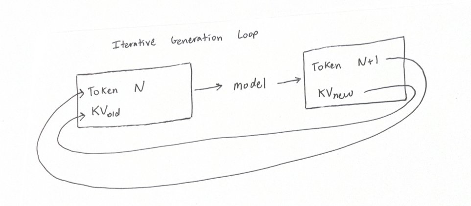
Old tokens + KV is fed through the model to predict the new token and KV. This is done in an iterative loop to keep generating next tokens. This loop needs to run even when reading the user's query (though the predicted next token is discarded).

Where token is the word outputted, and KV is the cumulative knowledge of the sentence that gets iteratively built up.

You should observe that generation is sequential. Token #50 depends on token #49 which depends on token #48 and so forth. This is why you see ChatGPT streaming one token generation at a time (autoregressively), and not in huge chunks of text. (If interested, learn more about causal masked attention and diffusion text models).

When trying to optimize LLMs to run on GPU hardware, we look at the most barebones operations that the GPU has:

• The compute: the amount of floating point math operations the GPU can compute, per second (FLOP/s)
• The memory bandwidth: the amount of bytes the GPU can load from the HBM VRAM into the SRAM / SMs (the actual compute cores)

We can naively calculate the amount of time a task takes as the sum of memory time + compute time. In this model, it seems like we should always try to optimize both the amount of compute and the bandwidth speed of GPUs.

In reality, GPUs are massively parallel processors. All the operations become interwoven between loading items and computing them, so with pipelining the wall-clock time can be approximated to just the time of the slower operation. The time taken to complete an operation really becomes:

In this model, we should focus on reducing the bottleneck and ensure that the time taken to load the weights is never more than the time to compute (never want to be memory bound).

The key number to watch is called arithmetic intensity: the amount of math being computed per byte loaded (kinda measuring the compute bound:memory bound ratio).

The roofline analysis model makes it easy to see:

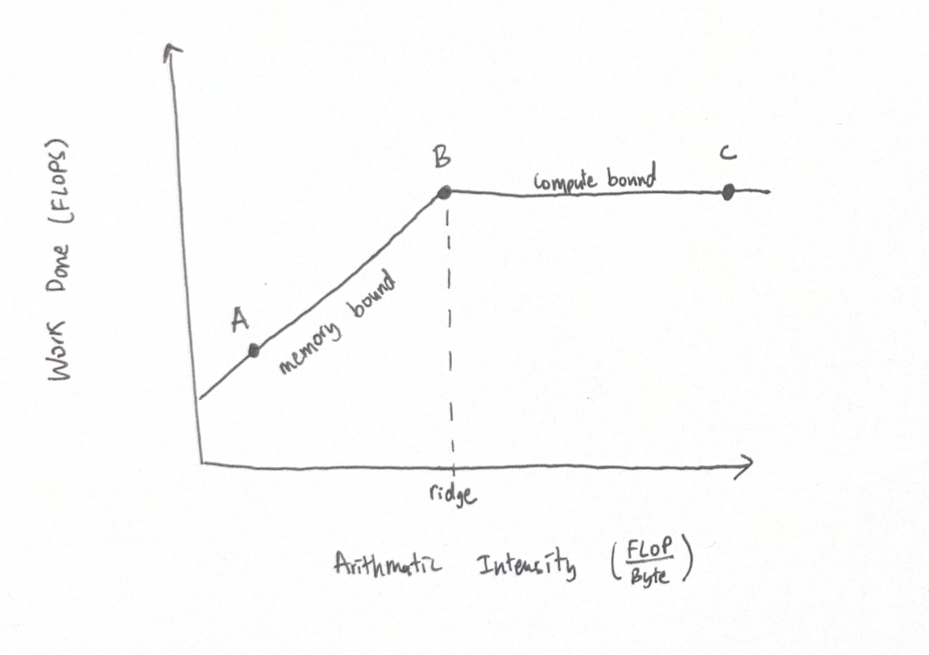
As arithmetic intensity increases, the amount of work done increases until you reach a point of being compute bound (memory is no longer the bottleneck). The horizontal axis is the arithmetic intensity and the vertical axis is the amount of usable work completed. You can see, as we increase the arithmetic intensity we can increase the amount of work done. This is because in the rising zone, we are memory bound, and improving the amount of compute that can be done per memory load increases total work. At a certain point, (the ridgepoint), we flip from being memory bound to compute bound. So, increasing the amount of work you can do per loaded byte doesn't improve anything since memory bandwidth is no longer the bottleneck.

At point A, we need to load the entire knowledge of the text and the model weights to create just 1 new token, then repeat it again. So, the arithmetic intensity is very low:

Our goal is to move toward point B, the ridgepoint, so we are optimally using all the compute we have available. So, our guiding question/goal is to move our traditional LLM processing from point A to point B by increasing arithmetic intensity, by primarily increasing the parallelism.

Parallelizing method 1: batch parallel

Two terms we need to clearly understand: Latency and throughput.

Latency is the time in between tokens per user. Having lower latency is better, since users see tokens faster.

Throughput is the total amount of tokens we produce per second. Having higher throughput is better because we are producing more tokens for more global users.

These don't always scale together. Increasing throughput may likely mean we make latency per user worse. For example, increasing concurrency (called batch size) often means that the latency is higher (worse) per user, while total throughput increases.

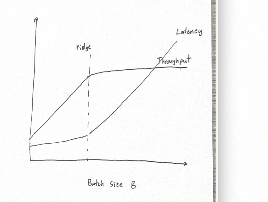
This graph shows the relationship between batch size and throughput and latency. By increasing batch size, we can parallelize and increase the arithmetic intensity, as shown by the equation below.

Since we increased the number of tokens by a factor of B and the divisor weight factor remained constant (shared weights amongst all batch members), we increased the arithmetic intensity. Batch size helps amortize the cost of loading the weights from HBM to SRAM/SMs.

In the above graph of batch size vs throughput, you'll see that it matches the roofline model since batch size increases arithmetic intensity. Latency also follows this model (just inverted, lower latency is better). To the left of the ridgepoint, latency gently increases because as batch size increases, the memory KV load increases (albeit at a slower rate than the total compute rising, due to the amortization of weights). To the right of the ridgepoint, we are now compute bound, and increasing batch size just increases the amount of work to be done linearly.

This also answers why we don't want to go to point C (all the way to the right in the roofline analysis chart). Going to point C is the same as point B (the ridgepoint) in terms of throughput (we can produce the same # of tokens, we are limited by the amount of compute we have!). However, latency (the individual user tokens per second) starts to suffer significantly.

There is another issue: GPUs are limited in memory capacity in the HBM. If we increase the batch size, we need more space to store the KV (memory is very expensive), which eventually runs out.

So while increasing batch size is a good trick we should be aware of:

• It does not amortize the cost of the KV loading (because KV is private to each sequence)
• It increases latency per user
• It cannot scale forever because of KV memory limits in HBM

Parallelizing method 2: sequence parallel

It is true that the mental model of sequential generation is always used in large language models. Even when the next token is known (for example, when parsing the input prompt), you still need to do the work (not to predict the next token, we already know what comes next) but so the model can create an internal representation to understand the input (the KV).

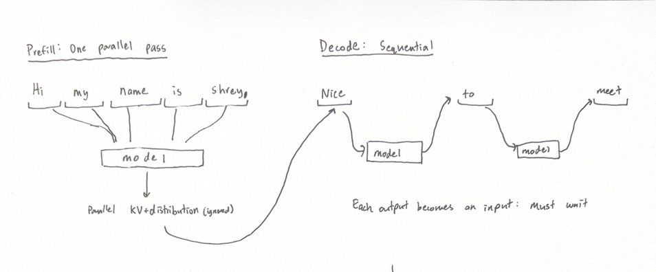
You can compute the probabilities of the next few tokens all at once, if you know what is coming next. For example, if I pass in 5 tokens at once "Hi my name is shrey," the model can generate the probabilities of each word AND the KV completely parallel. This first part of LLM inference (reading the input prompt) is called the prefill stage. It is fully parallelizable because every input token is already known, nothing is forcing the model to wait. It can shove the entire prompt at once and understand it using this sequence parallelism.

The generation of new tokens (decode) is what is sequential. Since we don't know the next token, we need to do the generation to repeat the loop with our predicted token. Each turn's input is the previous output, so we have to do one token per forward pass (low arithmetic intensity, memory bound), wasting idle GPU resources.

Let's do the arithmetic intensity math on the prefill. It is generating S sequence tokens, and loading in the weights + KV for that sequence. We can also combine sequence parallelism with batch parallelism, by outputting S*B tokens whilst loading 1 shared weights and a per batch KV.

So you can see that sequence parallelism amortizes not only the weights, but also the KV, since per each request the unique KV gets shared across the entire sequence. With batch parallelism, we could only amortize the weights.

One of the key components of the forward LLM pass is a method called attention. This is an O(n^2) operation, where each new token needs to attend to all the previous tokens. So, combining the parallelism of prefill with this O(n^2) operation very quickly makes prefill compute bound. Techniques like sparse attention reduce this O(n^2) component, but that's for another blog.

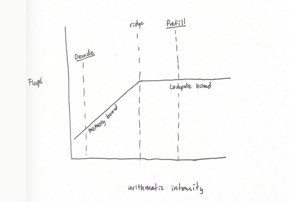
Batching and sequence parallel both climb the roofline, but batching only amortizes weights while sequence parallel amortizes the shared KV loading as well.

Speculating to get sequence parallelism during decode

The original paper by Leviathan '23 on speculative decoding can be found here.

We know that prefill can be parallelized, increasing arithmetic intensity, shifting from memory bound (bad) to compute bound (good). The question is how can we use this prefill verification trick during decode? The issue is that in prefill we knew the next tokens. We don't have a clue what's coming next in decode.

Leviathan solves this using a draft model, and borrows ideas from CPU speculative branching (guessing a branch before you know to prevent idling). The idea is simple: Before the target (main) model generates, run a tiny, fast, draft model which is autoregressively outputting tokens. I won't get into how the drafter is trained, but it's just trained to try to copy the main model. Since it's tiny, generating even 5 tokens is almost free and instant. Use these as the guess "next few tokens" so we can parallel verify.

The target model follows the prefill trick to verify all the draft tokens. At the first disagreement, the target can reject the draft's answer and keep its own. The last output of the verification pass is the prediction for the token in the n+1 position. In this way, we call this a +1 bonus token because the forward pass will always give us between 1 and n+1 correct tokens.

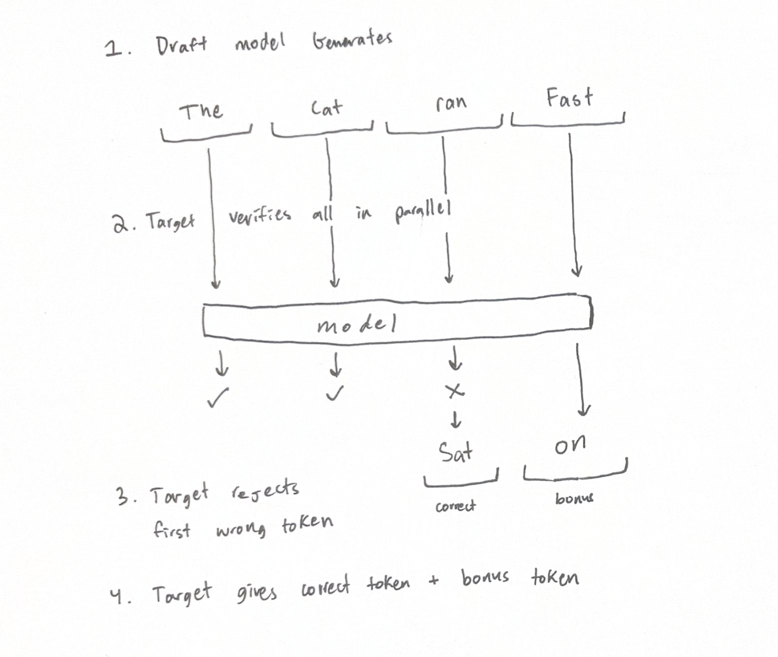
The number of tokens created has increased, while the bandwidth pressure remains constant:

This pushes us closer toward compute bound on the roofline analysis:

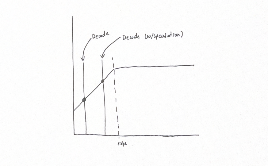
One stipulation: If we are running high enough batch size such that we are already compute bound before speculating, the additional cost of speculating comes as straight negative costs.

Costs (ignored when memory bound, paid heavily when already compute bound):

• Cost of verification -- the increase in arithmetic intensity cost linear with the amount of tokens we generated. In other words, even though 3x tokens speculated, 3x work done
• Cost of the speculator -- the cost of the actual speculation computed on the same GPU was straight loss!
• The latency of the speculator purely is additive to the total latency, because it runs before the actual verification pass

This is why it is important to balance the following, since they are all related in ways:

• The footprint of the speculator (don't want the speculator to use more than the free left over compute!)
• The acceptance rate / length of the speculator (too short/inaccurate, and the verification cost starts showing up!)
• The latency of the speculator
• Only running the speculator when you are memory bound, not compute bound

How does this drafter maintain the same distribution of the target?

Verification is a neat trick as well. Verification maintains that the final output has the exact same distribution as the target model through rejection sampling. All autoregressive models, (both the target and the drafter) output a distribution of probabilities as their prediction for the next token. So if your vocabulary was ["hi", "hello", "hey"], a model could output [.5, .3, .2] and a drafter could produce [.2, .7, .1] and so on. Generally, LLMs sample from this distribution using rules like temperature, top-k, top-p, etc in a random way.

Let's see how it plays out with speculation, with p(x) the target probability for token X, and q(x) as the draft probability for token X:

Case 1, p(x) > q(x): Drafter is less confident on its selected particular token than the target model, and we should always accept the drafter.

The intuition is that if we randomly sampled from the drafter, and picked something with a lower probability than the ground truth, we would've likely sampled the same token if we only had the target model anyway, and have no risk of over-representing relative to the target true distribution.

Case 2: p(x) < q(x): Drafter is overconfident on a selected particular token, and we should accept only p/q times, and for the rest, sample from the residual.

In this case, the drafter has put confidence on a part of the distribution that the target model would not have. This sounds like bad news, but realize, even the target may output tokens outside the top distribution sometimes. So, we accept the drafter p/q times. When we reject, 1-p/q, we sample from the residual distribution that the target wanted but the drafter put less probability mass on.

Here's an example:

Vocabulary = ["hi", "hello", "hey"]

The draft selected "hello," but the target would have only written "hello" 30% of the time. So, we accept "hello" .3/.7 = .43 times. On the remaining .57 times, we reject and sample from the residual:

And sample from this, so likely "hi."

Proving the same distribution

The probability of proposing q(x) and accepting min(1, p(x)/q(x)) together is below, and can be simplified by multiplying through:

The probability of something got proposed, rejected, then residual picked x:

Multiply out the first term and expand the definition of the residual:

which super cool cancels out to max(p(x)-q(x), 0) because p-q will be the same as q-p over the entire distribution (since p and q each sum to 1).

The total probability of picking token x is equal to the sum of the proposing and accepting, plus rejecting and residual:

This can be seen by trying both cases (p<q or q<=p) — we sum p + 0 or q + (p-q).

Using this really cool rejection sampling math, we mathematically guarantee a LOSSLESS identical distribution of output between accepted drafts and original target outputs.

Advances in speculators

I chose below a few papers that I found brought interesting advances to speculative decoding and highlight them grouped below. Leviathan's original speculative decoding worked and proved speculators as a concept, but the below papers have trained different architectures to lead to much higher speedups.

Better drafters

Medusa (Cai '24): Medusa finds that having an entirely separate drafter model can cause the drafter to drift off-policy from the target model. Instead of training a separate autoregressive model, it bolts on a few extra decoding heads on the last layer of the target model (after the main model is done training). The heads predict N+1, N+2, N+3 etc tokens ahead (1 token each). Found to have an up to 3.5x speedup on inference in coding workloads. The idea comes from MTP: a training technique where the model is told to predict multiple tokens ahead, so the model is forced to output tokens with long term thinking and not just the next statistically most probable token. The weakness of this model is that each head is independent. The head predicting N+2 is not knowledgeable of the N+1 prediction, which hurts the max acceptance rate / length of the model.

Eagle 1 (Li '24): Eagle found that simply bolting onto the last layer isn't enough. The key insight is that "the target knows best." This means the target model's hidden states already have a lot of context about the next few tokens, so we should use that, passing the model's features into the drafter. The acceptance rates jump ~5-10% compared to Medusa.

DFlash (Chen '26): As the above drafters got better and better, and the acceptance rate increased, people started increasing the amount of tokens generated by drafters, which increased the latency from the actual drafter. DFlash solves this by switching the model architecture of drafters from autoregressive to block diffusion models. Diffusion models denoise entire blocks of masked tokens in one forward pass, which causes hardly any increase in latency for longer text blocks, leading to a 6x lossless speedup. One weakness is that diffusion models generate each token somewhat independent of each other, so we get the same problem of Medusa/MTP showing up again.

Tree based verification

SpecInfer (Miao '23): In Leviathan's draft model, if the draft is wrong on a certain token, the entire sample has to be rejected after that point. In the case that the drafter is 50-50 uncertain on a certain token, the future tokens hinge on getting lucky at an earlier position. SpecInfer says: don't guess one sequence, guess a tree, branching into multiple continuations, and check them all. SpecInfer creates "tree attention," the method of checking all branches of the tree in parallel by only relating branches back to the parent's lineage when calculating the next token distribution.

Eagle 2 (Li '24): Eagle 2 adds tree based verification on top of Eagle 1. Furthermore, it creates dynamic trees: it goes deeper on branches with more confidence and wider/more shallow when less confident.

DDTree (Ringel '26): DDTree applies tree based verification to the DFlash diffusion block drafter. It is interesting to point out how the matrix sampling method works. The diffusion model outputs the probability of each token, and creates branches by sampling the most probable branch until the max prediction token limit is hit.

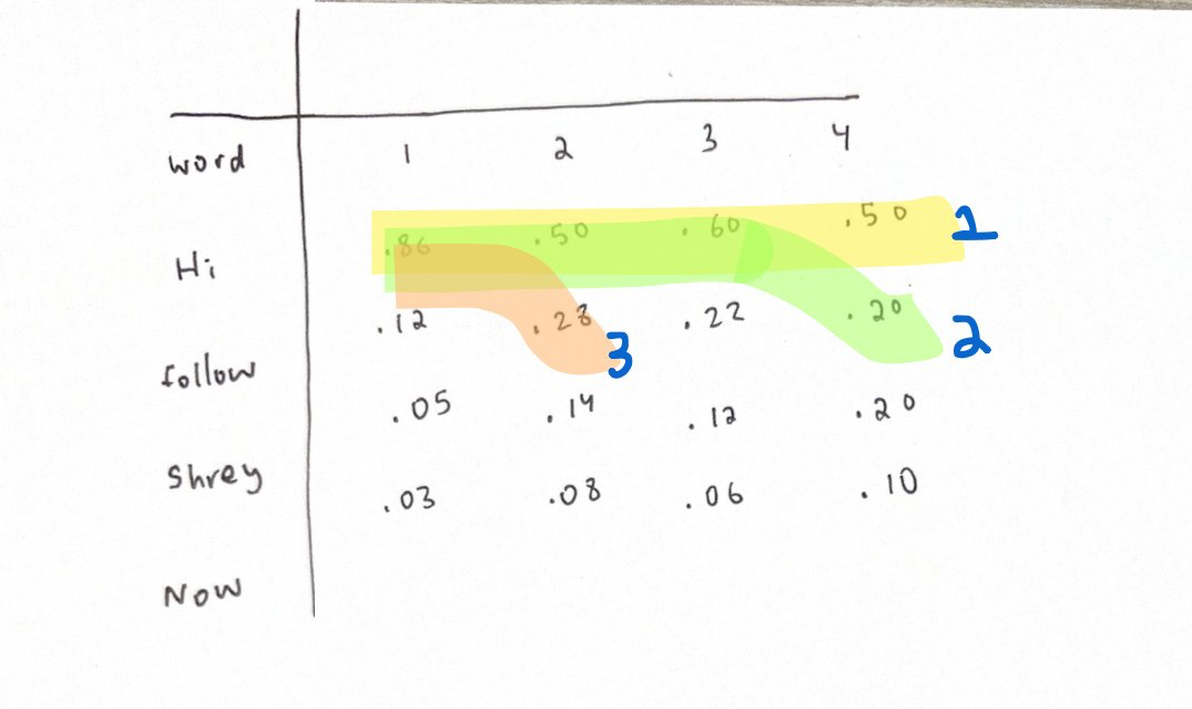
You can see above by multiplying the probabilities through the graph, we take the longest, highest probability branches first and stop going deeper as soon as a shorter branch has higher joint probability. This pushes speedups to 7-8x on certain workloads, and even at the same total token total as DFlash, has a higher speedup (because it can capture shallower paths that might've been missed by DFlash).

Some ideas on what's next

• Speculation to increase throughput, not latency: Speculation is typically used at lower batch sizes, when you are memory bound. But for long running agents, at longer context (KV) even large batch sizes flip to memory bound. This is an interesting blog by @togethercompute that uses speculative decoding (with the same target and draft model, just at limited KV size through a sliding window) to increase throughput 2x.
• Completely disaggregating the speculator: One of the costs we discussed was the cost of the speculator itself: it hogs memory bandwidth and compute. With chips like @taalas_inc and @Etched shifting toward more specialized inference, curious if we can use a specialized chip running a tiny model as a sidecar to the GPU running the target model.
• MoE speculation: Mixture of Experts is a type of model architecture where models only activate a small portion of total parameters per token, changing the landscape of memory vs compute. Routing aware drafters?
• Speculators that use MoE as an architecture themselves: As the target model becomes more and more experts, curious if the speculator itself becomes a tiny MoE? To help stay on policy.
• Routing to different speculators by workload: Code, general text, and data analysis have very different styles of text. Since the drafter is a tiny model, specialization improves the quality. Perhaps routing and tuning to a specific drafter after the prefill (using a linear layer head on the KV of the final token to classify?) could improve the accepted token length.
• Online training of speculators for zero data retention + hidden states already on hand: Training speculators requires having on-policy data (data that has been run through the target model for the hidden states + final correct output), as well as permission from customers to train on such data. @baseten has published some cool work showing you can train a speculator whilst serving the target model to customers, with the data never leaving the RAM and not affecting production latency. @modal is also working on specialized speculators per customer workload.

DSpark (DeepSeek '26): The newest DeepSeek speculative decoding paper. Improves upon DDTree. It's at the top of my reading list!

Thanks for reading! Thanks to @tejasybhakta and @charles_irl for all the help answering my questions learning about this topic! I started learning about LLMs and speculation just recently, so please correct any mistakes I made, I really would love to learn more. I wrote this as a forcing function (as Charles would say) to formalize my intuition on speculative decoding.