Making An Inference engine entirely in cpp (jwLLM part 1)
Intro and motivation
This semester I’m taking Linear Algebra, Operating Systems, and Cpp programming at UT Austin. I thought to myself, what better way to reinforce the learnings from the courses than to work on a semester long project that specifically focuses on the stuff I just learned from class?
I landed on building an inference engine in cpp to run GPT-2. Not only is it a super cool and fast growing field that I’m super interested in, It’ll almost perfectly map concepts from class to the project. Some things I’m looking forward to building and learning are:
- Learning how virtual memory works and seeing how we can implement that for KV (vLLM)
- Learning about matrix ops in lin alg and seeing how things like tensor parallel or efficient matrix mult can be performed
- Learning about mmap and seeing how we can use it to multiprocessor with fork() and to manage shared KV cache
- Learning about cache and how we can optimize our code (stride access patterns etc)
- Learning about CPU scheduling algos and seeing how we can build a scheduler for forward passes and also at macro, the GPU routing algos
- Learning Cpp tricks and tips and implementing them
- Learning how data is stored and floating point is represented in memory and seeing how quantization can be built
- Learning how efficient I/O is built and seeing how we can build things like FlexGen or SSD weight streaming
- Learning concurrent programming and seeing how we can speed up our inference server
- Learning networking and seeing how that can be applied to prefill decode disag
One thing I’d like to note: The goal of this project is to learn, not to showcase a project. If I wanted to, most of this could be completed with a LLM very quickly. Instead of focusing on learning, the projects are slow and intentional, so bear with me!
The code for this project can be found here: https://github.com/jwlaboratory/jwLLM
Making it just work
Before we get to do any of the cool optimizations; we must make the engine work (albeit slow!). Here’s a end demo of what we’ll have running by the end of this blog:
Let’s look at the overall architecture we need to implement to guide us:
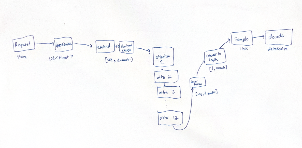
As you can see, it’s a long process, so onwards! Let’s start with the tokenizer.
Tokenizer
Let’s trace the data throughout generation, starting with the user request as a string. Since the model can only operate on numbers, we must convert the user query into a list of numbers. It seems trivial but actually was super painful to build. The code for the tokenizer is below, but I want to highlight the codepoint/utf-8/unicode translation and the merge priority system.
#include "tokenizer.hpp"
#include "matrix.hpp"
#include <fstream>
#include <iostream>
#include <nlohmann/json.hpp>

using json = nlohmann::json;

using namespace std;

Tokenizer::Tokenizer(string _mapping_json_path, string _merge_txt_path)
{
   ifstream f(_mapping_json_path);
   if (!f.is_open())
   {
       throw runtime_error("could not open mapping");
   };

   json j;
   f >> j;

   for (auto &[key, value] : j.items())
   {
       int id = value.get<int>();
       sToT[key] = id;
       tToS[id] = key;
   }
   f.close();

   // merge list
   ifstream merge_f(_merge_txt_path);
   if (!merge_f.is_open())
   {
       throw runtime_error("could not open merge path");
   }

   string merge_line;
   int cur_priority = 0;
   while (getline(merge_f, merge_line))
   {
       // Output the text from the file
       merge_priority[merge_line] = cur_priority;
       cur_priority += 1;
   }
   merge_f.close();
   regex_splitter = std::regex(R"('s|'t|'re|'ve|'m|'ll|'d| ?[a-zA-Z]+| ?[0-9]+| ?[^\s\w]+|\s+(?!\S)|\s+)");

   // unordered_map<int, char32_t> byte2unicode_data;
   // unordered_map<char32_t, int> unicode2byte_data;
   byte2unicode();
}

std::vector<int> Tokenizer::encode(string in)
{
   std::vector<int> final_tokens;

   // 1 apply the regex
   std::vector<std::string> split_input_string = regex_split(in, regex_splitter);

   for (std::string chunk : split_input_string)
   {
       // run per chunk the tokenization

       std::vector<int> tokenized_chunk = tokenize_chunk(chunk);

       for (int tokenized_chunk_nums : tokenized_chunk)
       {
           final_tokens.push_back(tokenized_chunk_nums);
       }
   }
   return final_tokens;
}

std::vector<int> Tokenizer::tokenize_chunk(std::string chunk)
{
   // we should keep a priority queue that keeps the adjacent tokens and the score
   // -> put closest 2 together, lookup
   // -> keep scores : arraypos1, arraypos2
   // -> after loop, merge lowest score, delete extra entry in array or mark it as no longer used (so its skipped)
   // complete until no more scores

   // struct MergeCandidate
   // {
   //     int priority_score;
   //     string str;
   // };

   // vector<struct MergeCandidate> all_candidates;

   // for (int i = 0; i < chunk.size() - 1; i++)
   // {
   //     std::string candidate_as_string = chunk[i] + " " + chunk[i + 1];

   //     int prio;
   //     if (merge_priority.find(candidate_as_string) == merge_priority.end())
   //     {
   //         prio = -1;
   //     }
   //     else
   //     {
   //         prio = merge_priority[candidate_as_string];
   //     }

   //     struct MergeCandidate candidate = {.priority_score = prio, .str = candidate_as_string};
   //     all_candidates.push_back(candidate);
   // }

   // // main loop
   // bool finished_merges = false;

   // while (!finished_merges)
   // {
   //     int lowest_prio = 9999;
   //     int lowest_prio_index = -1;

   //     for (int i = 0; i < all_candidates.size(); i++)
   //     {
   //         if (all_candidates[i].priority_score != -1 && all_candidates[i].priority_score < lowest_prio)
   //         {
   //             lowest_prio = all_candidates[i].priority_score;
   //             lowest_prio_index = i;
   //         }
   //     }

   //     // now we want to check
   //     if (lowest_prio_index == -1)
   //     {
   //         finished_merges = true;
   //         break;
   //     }
   //     else
   //     {
   //         // here we have at least one merge to make

   //         // case 1: first token
   //         if (lowest_prio_index == 0)
   //         {
   //             // delete this, update index lowest_prio_index+1
   //             all_candidates[lowest_prio_index + 1].left_token_left_index = all_candidates[lowest_prio_index].left_token_left_index;
   //             // reindex

   //             all_candidates[lowest_prio_index + 1].priority_score = new_prio;

   //             all_candidates.erase(all_candidates.begin() + lowest_prio_index);
   //         }
   //         else if (lowest_prio_index == all_candidates.size() - 1)
   //         {
   //             // last index case
   //             all_candidates[lowest_prio_index - 1].right_index_right_index = all_candidates[lowest_prio_index].right_index_right_index;
   //             all_candidates.erase(all_candidates.begin() + lowest_prio_index);
   //         }
   //         else
   //         {
   //             // normal case
   //         }

   //         // #, #, #, #
   //         // a, b, c, d
   //         // a-b, b-c, c-d
   //         // bc is lowest. then itll be a-bc, bc-d
   //         // if cd is lowest. then itll be a-b, b-cd
   //         // if ab is lowest. then itll be ab-c, c-d
   //     }
   // }

   // lookup each token

   // return final answ;

   std::vector<std::string> symbols;
   for (size_t i = 0; i < chunk.size(); i++)
   {

       unsigned char b = (unsigned char)chunk[i];
       // unsighend so bytes > 127 dont break
       char32_t cp = byte2unicode_data[b];
       // here we get the value correctly, if it was unsafe number, it gets re routed to a safe number
       // we now gotta make it back into a utf8
       symbols.push_back(codepoint_to_utf8(cp));
   }

   while (symbols.size() > 1)
   {
       // find lowest score index
       int lowest_index = -1;
       int lowest_pri = 9999999;

       for (size_t i = 0; i < symbols.size() - 1; i++)
       {
           string candidate = symbols[i] + " " + symbols[i + 1];

           int prio;
           if (merge_priority.find(candidate) != merge_priority.end())
           {
               prio = merge_priority[candidate];
               if (prio < lowest_pri)
               {
                   lowest_pri = prio;
                   lowest_index = i;
               }
           }
       }

       // if we found smth to merge, lets merge it
       if (lowest_index != -1)
       {
           symbols[lowest_index] = symbols[lowest_index] + symbols[lowest_index + 1];
           symbols.erase(symbols.begin() + lowest_index + 1);
       }
       else
       {
           // we need to break, no more merges
           break;
       }
   }

   // now we need to get the actual mapped indexes and return them
   std::vector<int> output;

   for (string symb : symbols)
   {
       output.push_back(sToT[symb]);
   }

   return output;
}

string Tokenizer::decode(std::vector<int> in)
{
   std::string disguised;

   for (auto &v : in)
       disguised += tToS.at(v);

   std::string raw;
   size_t i = 0;
   while (i < disguised.size())
   {
       unsigned char b = disguised[i];
       char32_t cp;
       size_t len;

       if ((b & 0x80) == 0x00) // 0xxxxxxx → 1 byte
       {
           cp = b;
           len = 1;
       }
       else // 110xxxxx 10xxxxxx → 2 bytes
       {
           cp = ((b & 0x1F) << 6) | (disguised[i + 1] & 0x3F);
           len = 2;
       }

       raw += (char)unicode2byte_data[cp];
       i += len;
   }
   return raw;
}

// from the internet: function to split into array based on regex
std::vector<std::string> Tokenizer::regex_split(const std::string &input, const std::regex &re)
{
   // Pass 0 instead of -1 to capture the actual regex matches (tokens)
   std::sregex_token_iterator first{input.begin(), input.end(), re, 0};
   std::sregex_token_iterator last;

   std::vector<std::string> tokens;
   for (auto it = first; it != last; ++it)
   {
       if (!it->str().empty())
       {
           tokens.push_back(*it);
       }
   }
   return tokens;
}

void Tokenizer::byte2unicode()
{

   // these are NORMAL ranges, ie normal characters, and should maintain the same value
   for (int i = 33; i <= 126; ++i)
   {
       byte2unicode_data[i] = i;
       unicode2byte_data[i] = i;
   }
   for (int i = 161; i <= 172; ++i)
   {
       byte2unicode_data[i] = i;
       unicode2byte_data[i] = i;
   }
   for (int i = 174; i <= 255; ++i)
   {
       byte2unicode_data[i] = i;
       unicode2byte_data[i] = i;
   }

   // abnormal ranges
   int n = 0;
   for (int i = 0; i < 256; i++)
   {
       if (byte2unicode_data.find(i) == byte2unicode_data.end())
       {
           // we have a special case!
           byte2unicode_data[i] = n + 256; // we do this to avoid ascii and move it into a safe range
           unicode2byte_data[n + 256] = i;
           n++;
       }
   }
}

// _chr = unichr if sys.version_info[0] == 2 else chr
// bs = list(range(ord("!"), ord("~")+1))+list(range(ord("¡"), ord("¬")+1))+list(range(ord("®"), ord("ÿ")+1))
// cs = bs[:]
// n = 0
// for b in range(2**8):
//     if b not in bs:
//         bs.append(b)
//         cs.append(2**8+n)
//         n += 1
// cs = [_chr(n) for n in cs]
// return dict(zip(bs, cs))

// func copied from gpt.
// itll basically do this. if its a 1 byte, itll keep it. if its a 2byte according to the utf8 pattern (>)
// if its 2 byte, itll do the pattern utf8 wants for 2 byte. ie wraps with 11000000 and 10000000
std::string Tokenizer::codepoint_to_utf8(char32_t cp)
{
   std::string out;
   if (cp < 0x80)
   {
       out += (char)cp;
   }
   else
   {
       out += (char)(0xC0 | (cp >> 6));
       out += (char)(0x80 | (cp & 0x3F));
   }
   return out;
}
Codepoint Fiasco
Users can type many types of characters, including potentially blank or special characters such as new lines. This can be annoying for debugging with non-visible characters or accidentally outputting these types of characters, so the tokenizer does a unique mapping such that:
- All input items (emojis, etc) that may take multiple bytes are interpreted on byte at a time
- If they (when interpreted as one byte) are “nasty” (new line, white space, etc), they are added 256 to shift into a 2 byte known safe range. For example “ “ becomes “Ġ”.
The result is rather strange. Variable length encoded objects are reinterpreted as one byte, shifted, then reinterpreted. But it works to make all of the characters deterministically mapped to 256 options that are safe.
Merges
Each character, though has a token id mapping, is not well interpreted by the model. That's like a human trying to read characters by characters instead of words by words. So the tokenizer then merges the pairs of the most frequent subtokens repeatedly. Here’s an example:
| S | U | B | M | A | R | I | N | E |
|---|---|---|---|---|---|---|---|---|
| 1 | 2 | 3 | 4 | 5 | 6 | 7 | 8 | 9 |
You can see SUBMARINE with each character mapping to a token ID. Let’s perform the merges (which merge in the order of priority given).
Merge priorities (given, trained by frequencies in training set)
| Tok 1 | Tok 2 | Merge Priority |
|---|---|---|
| S | U | 1 |
| SU | B | 2 |
| U | B | 3 |
| M | A | 4 |
| R | I | 5 |
| I | N | 6 |
| RI | N | 7 |
| RIN | E | 8 |
| MA | RINE | 9 |
The tokenizer will repeatedly merge the top priority that exists in the given list of tokens. In this case, it’ll merge S-U, then SU-B, then M-A, then R-I, then RI-N, then RIN-E, then MA-RINE. Notice it skips U-B and I-N and never merges SUB-MARINE.
This is cool because it learns the most frequent merges and therefore can split where semantic meaning is most helpful. In this case, the submarine split clearly into sub (which means under) and marine (which means water). It allows the model to still understand, even if it's never seen a submarine, that the word represents under-water.
Embedding
#include "matrix.hpp"
#include "embedding.hpp"
using namespace std;

Embedding::Embedding(SafeTensors &weights)
{
   WORD_TOKEN_EMBEDDING = weights.get("wte.weight");
   WORD_POSITIONAL_EMBEDDING = weights.get("wpe.weight");
}

Matrix Embedding::tokenized_to_embed(const std::vector<int> &token_ids)
{
   // token_ids is a single sequence of vocab ids
   int d_model = WORD_TOKEN_EMBEDDING.cols;
   int seq_len = token_ids.size();
   std::vector<float> out(seq_len * d_model);

   for (int i = 0; i < seq_len; i++)
   {
       int token_id = token_ids[i];

       for (int g = 0; g < d_model; g++)
       {
           out[i * d_model + g] = WORD_TOKEN_EMBEDDING.data[token_id * d_model + g];
           // out is flat array, word_token embedding is also flat array
       }
   }

   return Matrix(seq_len, d_model, out);
}

void Embedding::apply_positional_encoding(Matrix &token_embeddings)
{
   // seq len rows
   // dmodel cols

   // WORD_POSITIONAL_EMBEDDING is a table of size: position rows, dmodel cols

   int seq_len = token_embeddings.rows;
   int dmodel = token_embeddings.cols;

   for (int i = 0; i < seq_len; i++)
   {
       for (int g = 0; g < token_embeddings.cols; g++)
       {
           token_embeddings.data[i * dmodel + g] += WORD_POSITIONAL_EMBEDDING.data[i * dmodel + g];
       }
   }
}
Our tokenizer gave us a vector of numbers representing the IDs of each token. Next we need to convert into embeddings such that something that will give us rich features of each token. The dimensions of this is called dmodel. We do this by looking up in a table for our token ID.
The embeddings tell the model the meaning of each token, but it tells the model nothing about the position of each token. For example, if the word yellow appears at the start and at the end of the sentence, this looks identical to the model. So next we apply an addition of a positional vector, unique per position but the same for all tokens, that internally uses sine and cosine to be rotatory in nature to represent the location of each word.
Now we have a [sequence x d_model] representation that contains information about the tokens, the meaning, and the location of each token.
The attention block
Next, this [sequence x d_model] representing the token goes through 12 back to back attention blocks. Let’s look at what this is:
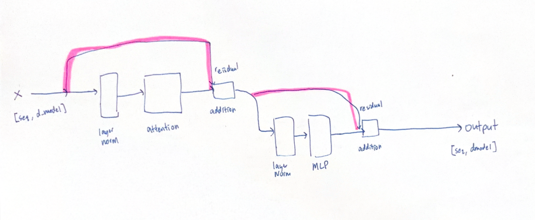
You’ll see the at each stage the dimensions remain the same (even though they may be internally transformed) from [seq, model]. You’ll also see this residual that keeps the original value summated throughout like a loop. Let’s dive into each piece we composed in this picture next.
Layer Norm
LayerNorm’s goal is to make all the data per row be standardized. It does this by normalizing each row to mean = 0, variance = 1, then scaling by gamma and shifting by beta. Eps is added to the denominator when making the variance zero to prevent dividing by zero. What helped me understand this part was remembering the Z-Score formula from high school stats.
// normalize each row to mean 0 / variance 1, then scale by gamma and shift by beta
Matrix Matrix::layernorm(const Matrix &gamma, const Matrix &beta, float eps) const
{

   vector<float> out(this->data.size());

   for (int i = 0; i < this->rows; i++)
   {

       // for each row
       float mean = 0;
       for (int g = 0; g < this->cols; g++)
       {
           mean += this->data[i * this->cols + g];
       }
       mean /= this->cols;

       float var = 0;
       for (int g = 0; g < this->cols; g++)
       {
           float diff = this->data[i * this->cols + g] - mean;
           var += diff * diff;
       }
       var /= this->cols;
       // vaiance is difference^2) averaged out
       // variance is sigma (standard deviation squared)

       // z sciore - (x-u)/sigma
       // we basically calcualting this

       // eps to pevent divide by zero

       for (int g = 0; g < this->cols; g++)
       {
           out[i * this->cols + g] = (this->data[i * this->cols + g] - mean) / std::sqrt(var + eps);
       }
   }

   // beta and gamma are learned so model decides what to expand. gamma is sscaler, beta is additive. //eps is to prevent divide by zero
   Matrix out_m = Matrix(this->rows, this->cols, out);
   return (out_m.broadcast_multiply_row(gamma)).broadcast_add_row(beta);
}
We run this layernorm constantly throughout the model, notably before each attention block.
Attention
Attention is the key work that makes this whole language model work. We first create Q, K, V, split by head, then do the self attention equation over each head, then finally concat.
I’m going to defer to a better source to explain the meaning and how this works internally. What really helped me was the video by Umar Jamil on transformers, found here: https://www.youtube.com/watch?v=ISNdQcPhsts and https://www.youtube.com/watch?v=bCz4OMemCcA
Matrix Attention::forward(const Matrix &x)
{
   // lets create k, q, v
   // fused multiplication intuition

   // x= 3x10 (3 seq len, dmodel=10)
   // fused = 10x10 but 3 stacked HORiZONTALLY, so its 10x30

   // output 10x30
   // Q = Y[:, 0:10] K = Y[:, 10:20] V = Y[:, 20:30]
   Matrix FusedQKV = (x.multiply(ATTENTION_WEIGHTS)).broadcast_add_row(ATTENTION_BIAS);

   Matrix Q = FusedQKV.slice_cols(0, dmodel);
   Matrix K = FusedQKV.slice_cols(dmodel, dmodel);
   Matrix V = FusedQKV.slice_cols(dmodel * 2, dmodel);
   // shape is [seqlen, d_model]

   // now, we need to do spliting
   int d_head = dmodel / heads;

   // say we have 4 heads and dmodel of 16
   // 0-4, 4-8, 8-12, 12-16
   // 0,   1,   2,    3
   Matrix output;
   for (int h = 0; h < heads; h++)
   {
       Matrix q_head = Q.slice_cols(h * d_head, d_head);
       Matrix k_head = K.slice_cols(h * d_head, d_head);
       Matrix v_head = V.slice_cols(h * d_head, d_head);
       // shape is [seq, dhead]

       // transpose k
       Matrix k_t = k_head.transpose(); //[dhead, seq]

       Matrix Q_kt = q_head.multiply(k_t); //[seq, seq]
       // tells us how much each entry in x relates to x, in that zone of embedding focus

       // divide by the sqrt d_k
       Matrix pre_mask = Q_kt.multiply_scalar(1 / std::sqrt(d_head));
       Matrix masked = pre_mask.mask_causal();
       Matrix softmaxed = masked.softmax_rows(); // still [seq, seq]

       Matrix post_v = softmaxed.multiply(v_head);
       // [seq,seq] * [seq, dhead]
       // now back to [seq, dhead]

       // append
       if (h == 0)
           output = post_v;

       else
           output = output.concat_cols(post_v);
   }

   // do the projections
   return output.multiply(PROJECTION_WEIGHTS).broadcast_add_row(PROJECTION_BIAS);
   //[seq, dmodel]
}I’ve also included the key code for the matrix helpers (slice_cols, concat_cols, and softmax) below, but they are pretty self explanatory.
Matrix Matrix::multiply(const Matrix &other) const
{
   // check dims
   if (cols != other.rows)
       throw std::invalid_argument("dims dont match");

   // do actual multiplication
   std::vector<float> out(rows * other.cols);

   for (int i = 0; i < this->rows; i++)
   {
       // for each row

       for (int q = 0; q < other.cols; q++)
       {
           // each col of the other now
           float sum = 0;
           for (int g = 0; g < this->cols; g++)
           {
               sum += this->data[i * this->cols + g] * other.data[g * other.cols + q];
           }

           out[i * other.cols + q] = sum;
       }
   }

   return Matrix(rows, other.cols, out);
}

Matrix Matrix::addition(const Matrix &other) const
{
   // check dims
   if (cols != other.cols || rows != other.rows)
       throw std::invalid_argument("dims dont match");

   // do actual addition
   std::vector<float> out(data.size());
   for (int i = 0; i < data.size(); i++)
   {
       out[i] = this->data[i] + other.data[i];
   }

   return Matrix(rows, cols, out);
}

Matrix Matrix::transpose() const
{
   // we store row x col
   // we need to swap to col x row

   // ie transpose:
   // [a,b,c,d,e,f]
   // 2x3 --> 3x2
   //[a, d, b, e, c, f]

   // 0,1 --> 1,0
   //

   vector<float> out(this->data.size());
   for (int i = 0; i < this->rows; i++)
   {
       for (int g = 0; g < this->cols; g++)
       {
           int newRow = g;
           int newCol = i;
           int total_per_row_new = this->rows;

           out[newRow * total_per_row_new + newCol] = this->data[i * this->cols + g];
       }
   }
   return Matrix(this->cols, this->rows, out);
}

Matrix Matrix::multiply_scalar(float scalar) const
{
   vector<float> out(this->data.size());
   for (int i = 0; i < this->data.size(); i++)
   {
       out[i] = this->data[i] * scalar;
   }
   return Matrix(this->rows, this->cols, out);
}

Matrix Matrix::gelu() const
{
   vector<float> out(this->data.size());
   for (int i = 0; i < this->data.size(); i++)
   {
       float x = this->data[i];
       out[i] = 0.5f * x * (1.0f + std::tanh(0.7978845608f * (x + 0.044715f * x * x * x)));
   }
   return Matrix(this->rows, this->cols, out);
}

Matrix Matrix::broadcast_add_row(const Matrix &row) const
{
   // we have a matrix [seqlen x dmodel]
   // we want to add a bias of size [dmodel]
   // we broadcast so this adds to each row

   if (row.rows != 1 || this->cols != row.cols)
   {
       throw std::invalid_argument("to broadcast add, must be row size =1");
   }

   vector<float> out(this->data.size());

   for (int i = 0; i < this->rows; i++)
   {
       for (int g = 0; g < this->cols; g++)
       {
           out[i * this->cols + g] = this->data[i * this->cols + g] + row.data[g];
       }
   }
   return Matrix(this->rows, this->cols, out);
}

Matrix Matrix::broadcast_multiply_row(const Matrix &row) const
{
   if (row.rows != 1 || this->cols != row.cols)
   {
       throw std::invalid_argument("to broadcast add, must be row size =1");
   }

   vector<float> out(this->data.size());

   for (int i = 0; i < this->rows; i++)
   {
       for (int g = 0; g < this->cols; g++)
       {
           out[i * this->cols + g] = this->data[i * this->cols + g] * row.data[g];
       }
   }
   return Matrix(this->rows, this->cols, out);
}

Matrix Matrix::softmax_rows() const
{

   vector<float> out(this->data.size());

   // loop 0: for each row
   for (int row = 0; row < this->rows; row++)
   {

       // loop one: find max val in the row
       float max = this->data[row * this->cols + 0];
       for (int g = 0; g < this->cols; g++)
       {
           if (this->data[row * this->cols + g] > max)
           {
               max = this->data[row * this->cols + g];
           }
       }

       // loop 2: calc sum and set each index to the e^(si-max)
       float sum_of_all = 0;
       for (int g = 0; g < this->cols; g++)
       {
           out[row * this->cols + g] = std::exp(this->data[row * this->cols + g] - max);
           sum_of_all += out[row * this->cols + g];
       }

       // loop 3: divide all by sum
       for (int g = 0; g < this->cols; g++)
       {
           out[row * this->cols + g] /= sum_of_all;
       }
   }

   return Matrix(this->rows, this->cols, out);
}

// given a matrix, give the data in col start, start+1, start+2... start+len
Matrix Matrix::slice_cols(int start, int len) const
{
   if (start < 0 || len <= 0 || start + len > this->cols)
       throw std::invalid_argument("slice out of range");

   vector<float> out(this->rows * len);
   int index = 0;
   for (int i = 0; i < this->rows; i++)
   {
       for (int g = 0; g < this->cols; g++)
       {
           if (start <= g && g < start + len)
           {
               out[index] = this->data[i * this->cols + g];
               index++;
           }
       }
   }
   return Matrix(this->rows, len, out);
}

Matrix Matrix::concat_cols(const Matrix &other) const
{

   if (other.rows != this->rows)
   {
       throw std::invalid_argument("got to have same rows for concat");
   }

   vector<float> out(this->data.size() + other.data.size());
   int max_len = this->cols + other.cols;

   for (int i = 0; i < this->rows; i++)
   {
       for (int g = 0; g < max_len; g++)
       {
           if (g < this->cols)
           {
               out[i * max_len + g] = this->data[i * this->cols + g];
           }
           else
           {
               out[i * max_len + g] = other.data[i * other.cols + g - this->cols];
           }
       }
   }
   return Matrix(this->rows, max_len, out);
}
// normalize each row to mean 0 / variance 1, then scale by gamma and shift by beta
Matrix Matrix::layernorm(const Matrix &gamma, const Matrix &beta, float eps) const
{

   vector<float> out(this->data.size());

   for (int i = 0; i < this->rows; i++)
   {

       // for each row
       float mean = 0;
       for (int g = 0; g < this->cols; g++)
       {
           mean += this->data[i * this->cols + g];
       }
       mean /= this->cols;

       float var = 0;
       for (int g = 0; g < this->cols; g++)
       {
           float diff = this->data[i * this->cols + g] - mean;
           var += diff * diff;
       }
       var /= this->cols;
       // vaiance is difference^2) averaged out
       // variance is sigma (standard deviation squared)

       // z sciore - (x-u)/sigma
       // we basically calcualting this

       // eps to pevent divide by zero

       for (int g = 0; g < this->cols; g++)
       {
           out[i * this->cols + g] = (this->data[i * this->cols + g] - mean) / std::sqrt(var + eps);
       }
   }

   // beta and gamma are learned so model decides what to expand. gamma is sscaler, beta is additive. //eps is to prevent divide by zero
   Matrix out_m = Matrix(this->rows, this->cols, out);
   return (out_m.broadcast_multiply_row(gamma)).broadcast_add_row(beta);
}

Matrix Matrix::mask_causal(float big_negative) const
{
   vector<float> out(this->data.size());

   if (this->rows != this->cols)
   {
       throw std::invalid_argument("must be a square matrix");
   }

   for (int i = 0; i < this->rows; i++)
   {
       for (int g = 0; g < this->cols; g++)
       {

           if (g > i)
               out[i * this->cols + g] = big_negative;
           else
               out[i * this->cols + g] = this->data[i * this->cols + g];
       }
   }
   return Matrix(this->rows, this->cols, out);
}MLP
The MLP (multi layer perceptron) is the next part in the transformer block. People commonly think the transformer is all the weights of the model, but in reality this part contains a huge amount of the compute and weights.
The MLP takes the incoming data, projects into a higher dimensionality, applies a non linearity, then projects back into the small space.
What made me understand this was thinking about how low rank factorization worked (which I wrote about here), and how this inverses it to get better (instead of less) control of how data can be separated.
#include "mlp.hpp"
#include <stdexcept>

MLP::MLP(SafeTensors &weights, const std::string &prefix)
{
   FC_WEIGHTS = weights.get(prefix + "mlp.c_fc.weight");
   FC_BIAS = weights.get(prefix + "mlp.c_fc.bias");
   PROJECTION_WEIGHTS = weights.get(prefix + "mlp.c_proj.weight");
   PROJECTION_BIAS = weights.get(prefix + "mlp.c_proj.bias");
}

Matrix MLP::forward(const Matrix &x) const
{
   //[seq, dmodel]

   // same idea as  low rank facotirzation But INVERSED. we project into big zone so we can seperate, then project done
   Matrix widened = x.multiply(FC_WEIGHTS).broadcast_add_row(FC_BIAS);

   widened = widened.gelu();

   Matrix shrunk = widened.multiply(PROJECTION_WEIGHTS).broadcast_add_row(PROJECTION_BIAS);

   return shrunk;

   // note. a LOT OF THE PARAMS live here. this is a HEAVY spot, very important
   // without non linearity this would be waste of time
}
Convert to logits, sample, and decode
The final part! We need to take this [seq, d_model] and turn it into something that is useful, the next token!
Recall at the start we indexed the tokid:embedding table. Now, we multiply by the transpose of the embedding table [dmodel, vocab], to get a table that shows [seq, vocab]. The last row tells us the scores of each vocab[i] position!
We sample from this (you can use things like temperature, top-p, nucleus, etc) but in this simple case we use argmax to get the top score and greedily decode it. We convert it back to a string and output it.
Matrix GPT::forward(const std::vector<int> &token_ids)
{
   if (token_ids.empty())
   {
       throw std::invalid_argument("forward needs at least one token");
   }

   // [seq, dmodel]
   Matrix x = embedding.tokenized_to_embed(token_ids);
   embedding.apply_positional_encoding(x);

   for (TransformerBlock &block : blocks)
   {
       x = block.forward(x);
   }

   x = x.layernorm(LN_F_WEIGHT, LN_F_BIAS);
   return x.multiply(WTE_T); // back to vocab size
}

int GPT::next_token(const std::vector<int> &token_ids)
{
   Matrix logits = forward(token_ids);

   // arg max for now
   int last = (logits.rows - 1) * logits.cols;
   int best = 0;
   for (int j = 1; j < logits.cols; j++)
   {
       if (logits.data[last + j] > logits.data[last + best])
       {
           best = j;
       }
   }
   return best;
}

std::vector<int> GPT::generate(std::vector<int> token_ids, int max_new)
{
   for (int i = 0; i < max_new; i++)
   {
       if ((int)token_ids.size() >= MAX_POSITIONS)
       {
           break;
       }
       int next = next_token(token_ids);
       if (next == EOT_TOKEN)
       {
           break;
       }
       token_ids.push_back(next);
   }
   return token_ids;
}Fin
Obviously a lot of optimizations can be built next, which is exactly what we will be doing next! Stay peeled to watch for the next blog in this series.